9 How to Train and Use Deep Learning Models in Microscopy

Practical considerations through the lens of segmentation

Authors

Affiliations

Joanna W. Pylvänäinen

Turku Bioscience Centre, University of Turku and Åbo Akademi University

Faculty of Science and Engineering, Cell Biology, Åbo Akademi University

InFLAMES Research Flagship Center, University of Turku

Iván Hidalgo-Cenalmor

Turku Bioscience Centre, University of Turku and Åbo Akademi University

Faculty of Science and Engineering, Cell Biology, Åbo Akademi University

InFLAMES Research Flagship Center, University of Turku

Guillaume Jacquemet

Turku Bioscience Centre, University of Turku and Åbo Akademi University

Faculty of Science and Engineering, Cell Biology, Åbo Akademi University

InFLAMES Research Flagship Center, University of Turku

Turku Bioimaging, University of Turku and Åbo Akademi University

9.1 Introduction

9.1.1 The challenge

The growing volume and complexity of image data necessitate increasingly advanced analytical tools. One example of challenging tasks is image segmentation, the process of identifying and delineating structures of interest within images. Segmentation can be particularly difficult and time-consuming when dealing with large, multidimensional datasets, such as 3D volumes or time-lapse sequences, where manual annotation becomes impractical. Machine learning (ML), especially deep learning (DL), can provide effective solutions to these challenges¹.

ML algorithms learn patterns from data to perform tasks such as image classification and segmentation. Traditional ML methods, like random forest classifiers, depend on manually defined image features to classify pixels^2–4. In contrast, DL algorithms can automatically discover and extract relevant features directly from image data using multilayer neural networks, which eliminates the need for manual feature selection. DL techniques are widely applied in complex image analysis tasks, including segmentation, object detection, feature extraction, denoising, and restoration^5,6. Due to their ability to automatically learn hierarchical features, DL methods usually achieve greater accuracy and efficiency than traditional ML techniques^7,8.

Segmentation greatly benefits from ML and DL, as manual segmentation is extremely time-consuming and impractical for large datasets. This chapter offers practical guidance on preparing a segmentation project and emphasises effective DL applications to tackle these challenges. While we focus on segmentation as a case study, the principles, workflows, and considerations discussed here are broadly applicable to other image analysis tasks, such as classification or denoising. Readers interested in these areas can adapt the described approaches to their specific needs.

9.2 Preparing for your project

9.2.1 Defining your task and success criteria

Every image analysis project should begin by clearly defining the scientific question you wish to answer, along with the criteria by which success will be measured. These foundational decisions will fundamentally shape your entire workflow. Careful planning of your objectives ensures that the chosen approach closely aligns with your scientific goals and will guide critical decisions about data annotation, model selection and performance evaluation.

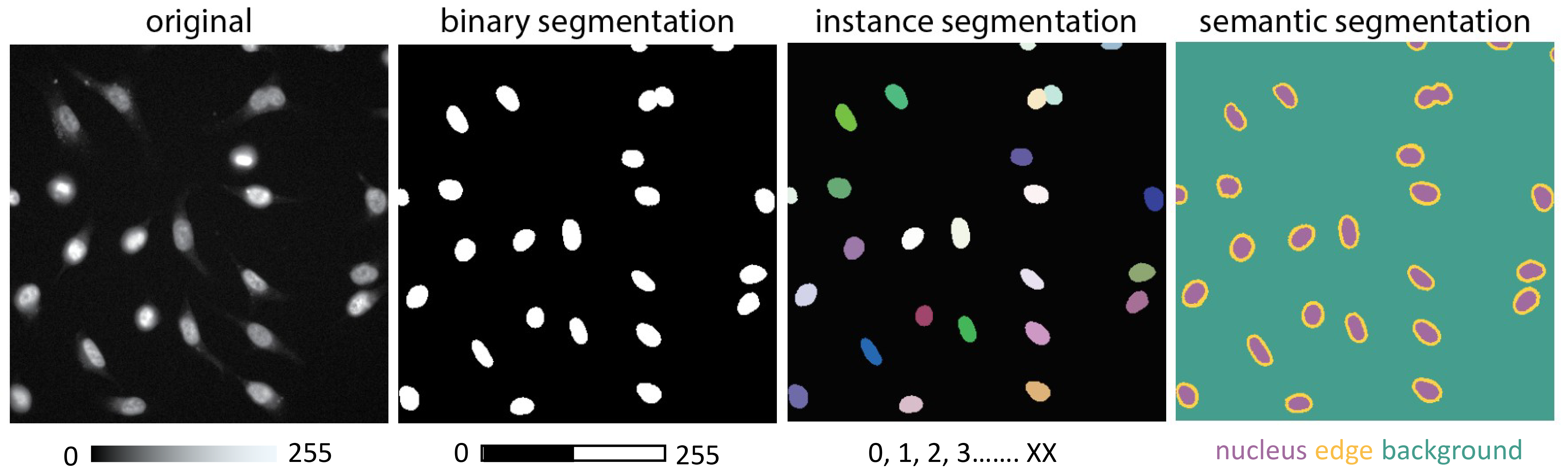
Since segmentation serves as the central example in this chapter, it is important to first understand the different types of segmentation tasks encountered in microscopy before discussing how deep learning methods can be applied. These tasks can typically be categorised into three main types (Figure 9.1). Each segmentation type presents distinct challenges and is suited to different biological questions:

Binary segmentation: This is the simplest form of segmentation that separates the foreground from the background. For example, in a microscopy image, this involves distinguishing cell nuclei (foreground) from the rest of the image (background). This method is useful for detecting whether a structure is present or absent without distinguishing individual objects.

Instance segmentation: This type of segmentation identifies and labels each object independently. For instance, each cell in an image obtains a unique label. This method is crucial for tracking individual cells over time or measuring specific characteristics of each cell separately.

Semantic segmentation: This segmentation strategy involves labelling every pixel in an image according to its class, such as “nucleus,” “cytoplasm,” or “background.” Unlike instance segmentation, semantic segmentation does not differentiate between individual objects within the same class. This method is beneficial for analysing the spatial relationships and distribution of various cellular components.

Figure 9.1: The three main types of segmentation in microscopy images. **original**: A raw grayscale fluorescence microscopy image showing cell nuclei stained with a nuclear marker. **binary segmentation**: Simplifies the image into two classes—foreground (white, nuclei) and background (black). **instance segmentation**: Assigns a unique label (shown in different colours) to each nucleus, facilitating individual object identification. **semantic segmentation**: Categorises each pixel into predefined classes—nucleus (purple), nucleus edge (yellow), and background (teal)—without distinguishing between individual objects.

Consider whether your segmentation solution is meant for a specific experiment or needs to generalise across various imaging techniques, sample types, or experimental conditions. Additionally, evaluate the volume of data to analyse, the feasibility of manual analysis, and the resources available to create a tailored image analysis pipeline. Avoid overengineering a solution when a simple analysis could provide the answer you seek.

Alongside task-specific considerations, it is equally important to clearly define the success criteria based on your objectives. For example, be prepared to answer the question, “What do I need to accomplish for my analysis to be sufficient?” – see Chapter 10 for more information. This is important because no analysis is ever 100% accurate. Establishing these criteria early streamlines both the development and evaluation processes, ensuring that your outcomes are scientifically meaningful and practically useful (see Chapter 10).

While the following steps focus on segmentation, the underlying principles can be readily adapted to a wide range of DL tasks in microscopy.

9.2.2 Evaluating alternatives: Is DL the right choice?

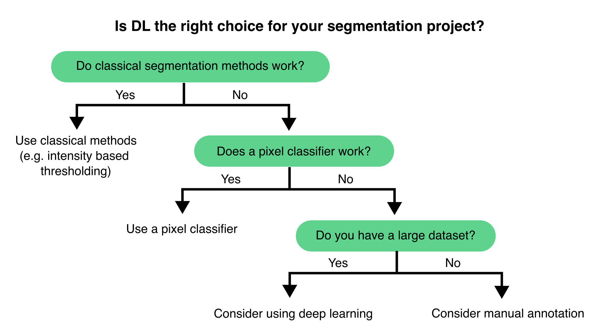
Figure 9.2: Is DL the right choice for your segmentation project? This decision tree guides the selection of appropriate segmentation approaches based on data complexity and project needs. Begin by testing classical image processing methods, such as intensity-based thresholding, which are efficient and easy to apply for well-defined features. If these methods prove insufficient, consider using a pixel classifier, which provides a user-friendly and effective solution for smaller datasets. Only consider DL if you possess a large annotated dataset and previous methods have failed. In the absence of suitable data or methods, manual annotation may be necessary.

Choosing the right computational method is essential for consistent and reproducible image analysis. For example in segmentation tasks, while DL can deliver exceptional segmentation performance, traditional methods and pixel classifiers still offer straightforward and efficient solutions for most tasks (Figure 9.2).

Traditional image processing techniques—such as intensity-based thresholding, morphological operations, edge detection, and filtering—are ideal for objects with clear, distinguishable features. These methods are well-documented, easy to understand, and usually require minimal computing resources. Pixel classifiers, in particular, are user-friendly and can efficiently tackle many segmentation challenges with minimal manual annotation, making them highly effective for simpler analyses or smaller datasets.

DL methods excel in complex scenarios where traditional approaches fail, especially when dealing with noisy or context-dependent data. When trained on large, annotated datasets, DL models can effectively generalise across diverse imaging conditions and sample types, rapidly processing significant volumes of images. However, in the absence of pre-trained models, DL methods rarely offer shortcuts for data analysis. DL methods generally take effort and time to implement.

If you are unsure which approach to use, we usually recommend first trying classical image processing methods and pixel classifiers (Figure 9.1). We typically initiate a DL project only if these methods fail to produce satisfactory results (see Section 9.3.3.2).

9.3 Implementing a DL segmentation workflow

Although we use segmentation as our primary example, the workflow outlined in this section can be adapted to other deep learning tasks in microscopy and bioimage analysis.

9.3.1 Overview of a typical DL segmentation workflow

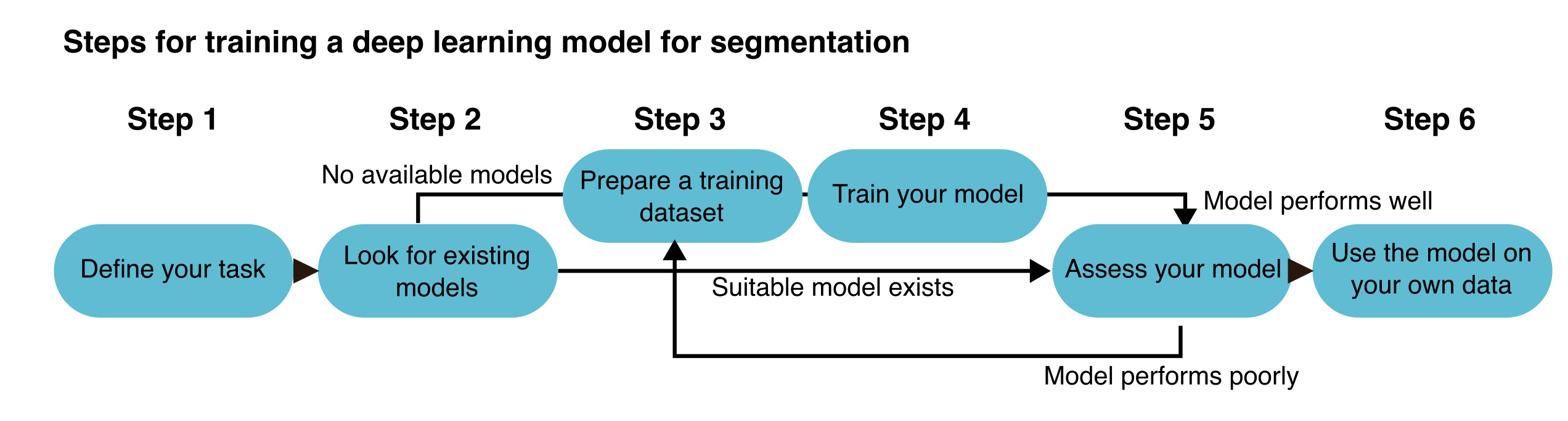
Once you decide to implement a DL approach for segmentation, the workflow can be divided into a series of steps (Figure 9.3).

The process starts by clearly defining your task (in this example, segmentation) and selecting the right DL approach (Step 1). Next, evaluate whether any existing pre-trained models can be used directly on your data or adapted for use (Step 2). If additional training is required—either from scratch or through transfer learning—prepare an appropriate training dataset that reflects your segmentation problem (Step 3). Then, train your model using the prepared dataset (Step 4) and thoroughly evaluate its performance using validation or test data (Step 5). Based on the results, you may need to refine the model by adjusting hyperparameters, improving annotations, or expanding the dataset. Once the model performs satisfactorily, it can be used to segment new, unseen data (Step 6). We will now discuss each step in more detail.

Figure 9.3: Conceptual workflow for training a DL segmentation model. The workflow begins with defining the segmentation task (Step 1), followed by searching for suitable pre-trained models (Step 2). If no such model exists, a training dataset must be prepared (Step 3), and the model is trained (Step 4). The trained model is then evaluated on validation or test data (Step 5). If it performs well, it can be applied to new data (Step 6); otherwise, the model is iteratively refined by returning to earlier steps. Feedback loops from evaluation to earlier stages help refine and improve the model accuracy.

9.3.2 Selecting a suitable DL approach

The first step in choosing a DL approach for image segmentation is to clearly define your segmentation task, whether it’s binary, semantic, or instance segmentation (Figure 9.1), and to determine if you require 2D or 3D segmentation. Next, you should consider whether the model or tool you plan to use makes assumptions about the shapes or structures of the objects you want to segment. Understanding these assumptions will aid in selecting a model that fits your specific biological problem (see Section 9.2.1). Additionally, consider the amount of data that needs annotation for a particular DL approach (see Section 9.3.4.5). Finally, take into account your available computational resources (see Section 9.4.2). More complex models typically demand more GPU memory, longer training times, and additional storage, especially for 3D data or large datasets.

For example, StarDist⁹, a widely used tool for nuclei segmentation, assumes that objects are star-convex polygons: i.e., a shape for which any two points on its boundary can be connected by a single line that does not intersect the boundary. This assumption works well for round or oval shapes but makes StarDist less suitable for segmenting irregularly shaped or elongated structures. In contrast, Cellpose¹⁰ uses spatial vector flows to direct pixels toward object centres. This approach enables Cellpose to segment objects of various shapes and sizes, including irregular, elongated, or non-convex forms.

Choosing the right DL strategy requires aligning your goal, object shape, data dimensionality, and computing capacity with the strengths and assumptions of the available DL architectures.

9.3.3 Deciding whether to train a new model

Figure 9.4: Decision workflow for selecting a DL model training approach. This flowchart outlines how to determine an appropriate training approach based on the availability and performance of pre-trained models.

9.3.3.1 Leveraging pre-trained models

The increasing availability of already trained (pre-trained) DL models has greatly simplified image analysis. Many of these models can be directly applied to your data, removing the need to train your own model^11,12. This reduces the technical barrier and saves time, making advanced analysis more accessible. However, it is essential to evaluate the quality of any pre-trained model before relying on its results (Figure 9.4). A model that performs well in one context may not be as effective on your specific data. Always conduct quality control by visually inspecting the outputs and assessing performance with quantitative metrics such as Intersection over Union (IoU) or F1-score, using a small, representative test set. This step is vital when model predictions are used in downstream analyses (see Section 9.3.7).

Another significant benefit of pre-trained models is their adaptability. Instead of starting from scratch, you can often fine-tune an existing model (see Section 9.3.6). This method entails retraining the model with a smaller, task-specific dataset, enabling it to adjust to your images while requiring far fewer annotations.

Several excellent resources host pre-trained models suitable for microscopy. Researchers also increasingly share trained models alongside their datasets and publications, promoting open science. Platforms like Zenodo are commonly used for this purpose^13,14, although deployment may require handling specific file formats or environments (see Chapter 8 for more information).

9.3.3.2 When to train your model

Pre-trained models serve as an excellent starting point for various microscopy tasks. However, there are many scenarios where training a custom model becomes essential. Custom training enables the model to learn the specific characteristics of your dataset, experiment, or imaging modality, resulting in enhanced performance^15–17. This is particularly crucial when your data differs significantly from the data used to train existing models. Thus, their performance should always be validated. If quality assessment metrics are poor or key features are not accurately segmented, consider training your own model.

Ultimately, always evaluate the model’s performance against your defined success criteria (see Section 9.3.7). Custom training may be the best path forward if the current model does not meet your needs.

9.3.4 Preparing your dataset for training

A well-designed training dataset is essential for developing successful DL models on tasks such as segmentation. The number of images and the quality of annotations needed vary based on factors such as task complexity and the architecture of the intended model.

9.3.4.1 Types of model training

For segmentation, most DL models are trained using supervised learning, where each input image is paired with a manually annotated ground truth mask. In this context, all objects that need segmentation must be annotated in the training dataset. This approach enables the model to learn a direct mapping from raw images to segmentation outputs (Figure 9.7).

However, alternative approaches can help reduce the need for extensive manual annotations:

Unsupervised learning trains models without paired input and output data. Instead, the network identifies patterns or similarities in unlabelled images¹⁸.
Self-supervised learning involves designing tasks in which the model learns useful features directly from the input data without needing explicit labels¹⁹.
Weakly supervised learning uses partial, noisy, or imprecise labels to guide training, which can significantly reduce annotation effort^20,21.

9.3.4.2 Creating Manual Annotations

Creating accurate annotations manually is time-consuming, particularly for 3D datasets. Tools like Fiji²², Napari²³, and QuPath²⁴ are frequently employed for manual labelling. Typically, manual annotation involves drawing each object on the image and converting it into a mask or label.

Here it is an example pipeline for manually annotating data using Fiji

See also¹³.

Open Fiji – activate the LOCI update site and restart Fiji.
LOCI tools are required for exporting ROI maps. To enable them, go to Help > Update > Manage Update Sites, look for ‘LOCI’ and check the Active checkbox. Then, click on Apply and Close and Apply Changes, this update site ensures the necessary plugins are installed. Finally, restart Fiji.
Open your image you wish to annotate.
Use File › Open to browse and load the microscopy image that you want to label manually. You can also drag and drop your image to Fiji.
Select the Oval or Freehand selection tool.
These tools, found in the Fiji toolbar, allow you to manually outline the structures of interest in your image.
Start drawing around each object (yes, each one!).
Carefully trace each cell or feature you want to annotate—precision is key to ensure useful training data for DL.
After drawing each object, press “t” on your keyboard → the selection will be stored in the ROI manager.
This adds the drawn region to the ROI (Region of Interest) list, keeping track of all annotated objects in the image.
Repeat until all objects are in the ROI manager.
Continue drawing and pressing “t” until you have annotated every relevant object in the image.
When finished, go to Plugins › LOCI › ROI Map.
This plugin converts all saved ROIs into a single labeled ROI map image, assigning unique values to each region.
Save the generated ROI map with the same title as the original image in a separate folder.
Consistent naming ensures each annotated map can be correctly matched with its corresponding raw image during training or analysis.
At the end, you will have one folder with the original images and another for the ROI maps.
This separation makes it easier to organise and use your data with image analysis or DL pipelines.

9.3.4.3 Accelerating annotation with automatic initial segmentations

Creating high-quality annotations often represents the most time-consuming aspect of training a DL model for segmentation. To alleviate this burden, you can start from automatically produced initial segmentations. For example, using simple thresholding methods such as Otsu’s thresholding to generate rough segmentations can decrease the total annotation time. Even more powerfully, pre-trained DL models such as those provided with StarDist⁹ and Cellpose¹⁰ can generate more accurate initial segmentations that users can manually refine. These annotations can then be used to retrain the model, establishing an iterative cycle that accelerates both labelling and model refinement.

New tools are also pushing the boundaries of interactive annotation. For example, Segment Anything for Microscopy (μSAM)¹⁵ facilitates automatic and user-guided segmentation and allows the model to be retrained on user-provided data. Similarly, Cellpose 2.0¹⁶ features a human-in-the-loop workflow, allowing users to edit DL-generated segmentations. This hybrid approach enhances accuracy while significantly reducing the time and effort required for manual annotation.

9.3.4.4 Expanding your dataset with augmentation and synthetic data

When the number of training samples is limited, augmentation techniques can enhance dataset diversity to improve the model’s generalisation ability and performance on validation and testing^25,26. Common augmentation strategies include image rotation, flipping, scaling, and contrast adjustment. However, it’s important to apply augmentation carefully, as excessive or unrealistic augmentation can confuse the model or cause it to learn patterns that do not exist in real data.

In the absence of sufficient real data, synthetic data generated through simulations or domain randomization can help pre-training a model^27,28. These synthetic samples can expose the model to a broader range of scenarios early in training, before transitioning to fine-tuning with real, annotated data.

In summary, a successful segmentation pipeline relies on a careful balance between data quantity and annotation quality. Augmentation strategies can efficiently help to scale and balance training datasets.

9.3.4.5 Choosing the dataset size: specific vs. general models

In supervised training, it is crucial that each image in the training set is accompanied by a corresponding label image (see Section 9.3.4.1). The number of image-label pairs required depends on the number of labels per image, the complexity of the model and the desired level of generalisability. Still, the key is having enough representative examples and corresponding annotations for the model to learn meaningful patterns.

Small and well-curated datasets consisting of tens of images may suffice for highly specific applications, such as segmenting cells or nuclei using a defined imaging modality¹⁷. In these scenarios, transfer learning can also be especially beneficial (see Section 9.3.6). Models designed to generalise across a wide range of conditions, tissue types, or imaging modalities typically require much larger and more diverse datasets (hundreds to thousands of annotated images)¹⁰. These datasets are essential for capturing the inherent variability in broader use cases.

9.3.5 Training a segmentation model from scratch

Once you have annotated your training dataset, the next steps are to organise your data for training, initialise your model by selecting appropriate hyperparameters, and start the training process (Figure 9.7).

9.3.5.1 Splitting your training data: training, validation, and test sets

A crucial part of preparing your dataset is dividing it into three subsets: training, validation, and test sets. Each subset should contain the original microscopy images paired with their corresponding ground truth segmentations. A common strategy is to allocate 70–80% of the data for training, 10–15% for validation, and the remainder for testing. To ensure unbiased evaluation, ensure these subsets do not overlap in terms of fields of view, represent the variability of your entire dataset, and are randomly assigned to each set respectively.

The training set is used to train the model to recognise relevant features. To enhance generalisation, it must encompass a broad spectrum of scenarios and image conditions. Otherwise, the model risks overfitting—excelling with the training data but faltering with new images (Figure 9.6).

The validation set is used during training to provide feedback on the model’s performance with unseen data. This feedback, conveyed as validation loss, assists in detecting overfitting (Figure 9.6), guiding hyperparameter tuning (see Section 9.3.5.3), and informing training decisions. Although a separate validation set is ideal, many workflows create one in practice by reserving a portion (typically 10% to 30%) of the training data.

The test set, which serves a separate role, evaluates the model’s performance on entirely unseen data. Unlike the validation set, the test set is not utilised during training, ensuring an unbiased performance assessment. Test images should also include ground truth annotations to facilitate quantitative quality control. Reporting test set performance, using metrics such as accuracy, IoU, or F1-score, is crucial, especially when publishing or benchmarking your model²⁹.

9.3.5.2 Understanding the training process

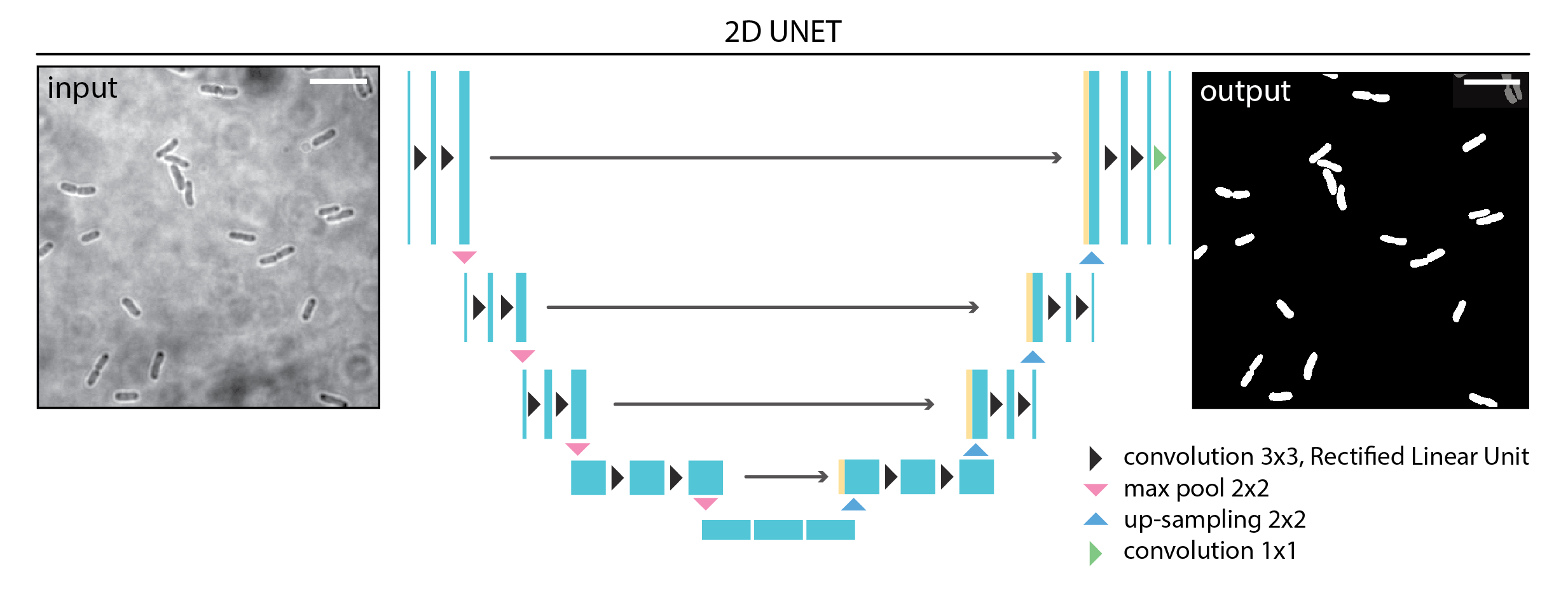
A DL model is composed of multiple layers (Figure 9.5). Each layer contains tens to hundreds of image processing operations (typically multiplications or convolutions), each controlled by multiple adjustable parameters (called weights). Altogether, a DL model may contain millions of adjustable weights. When an input image is processed by a DL model, it is sequentially processed by each layer until an output is generated. Segmentation tasks typically involve converting input images into labelled outputs. During training, the model weights are modified as the model learns how to perform a specific task.

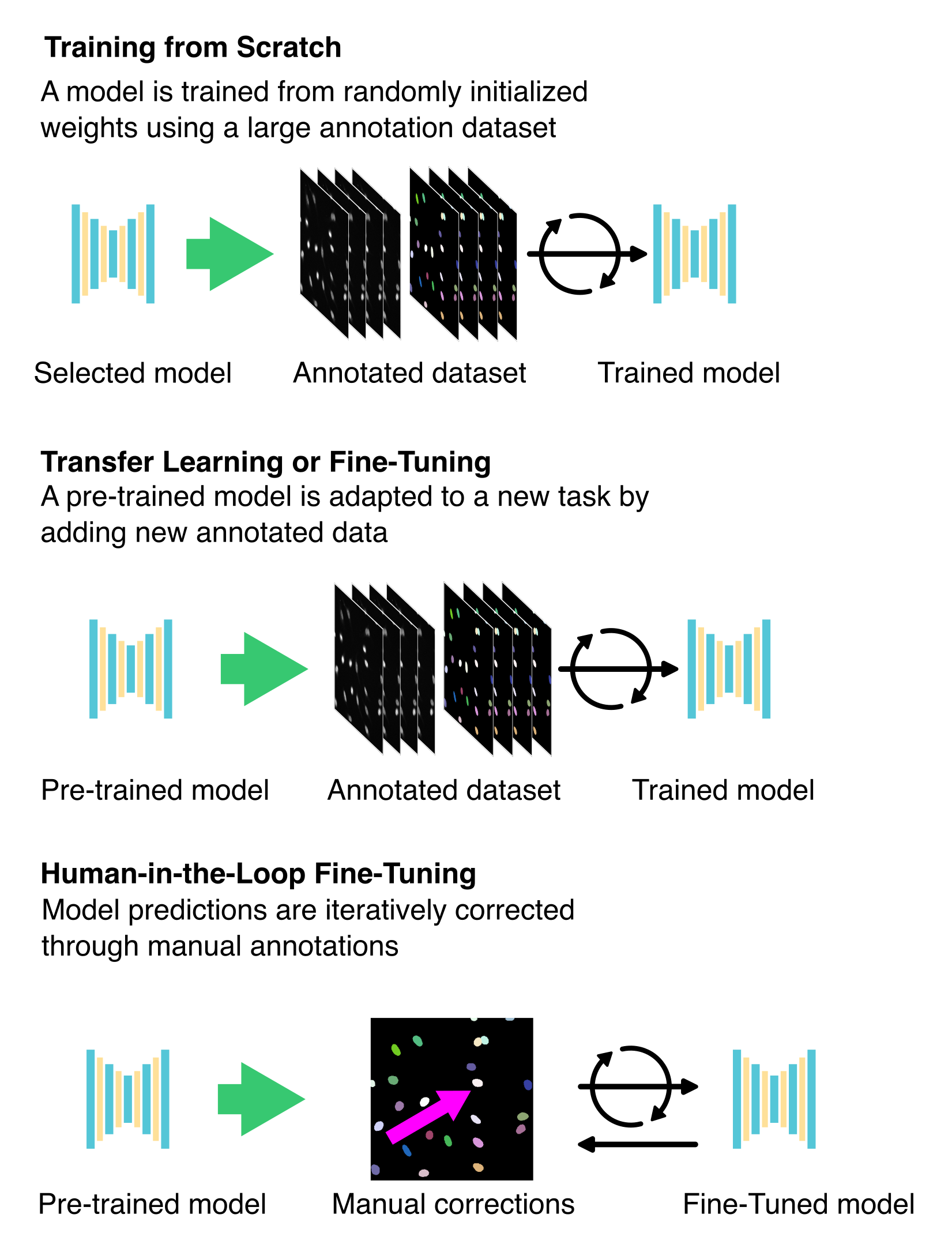
Figure 9.5: 2D U-Net architecture for image segmentation. It applies layers of convolutions, pooling, and upsampling to extract features and generate labelled segmentation masks. During training, model weights are iteratively adjusted based on the difference between predictions and ground truth labels, using a loss function and backpropagation.

Training begins with initialising these weights. When training from scratch, the initialisation is often random. However, when using a pre-trained model, the weights are already optimized based on previous training, providing the model with a significant head start (see Section 9.3.6).

The training process is iterative (Figure 9.7). Each cycle of training is called an epoch. During each epoch, the model typically learns from every image in the training set. Since datasets are often too large to fit into memory all at once, each epoch is divided into steps or iterations, with each step processing a smaller subset of the data known as a batch. The batch size determines how many samples are processed simultaneously.

During each step, the model generates predictions for the current data batch. These predictions are compared to the ground truth labels using a loss function that calculates the similarity between the predictions and the ground truths. This score is called the training loss. The model utilises this feedback to adjust its weights through a process known as backpropagation, guided by an optimisation algorithm, to improve its accuracy in future iterations.

At the end of each epoch, the model assesses its performance on the validation set, which comprises data it has not encountered during training. This produces the validation loss, indicating how well the model generalises to new data.

Monitoring both training and validation losses during training helps determine whether the model is learning effectively. A consistently decreasing validation loss indicates that the model is improving and generalising well (see Section 9.3.5.4).

9.3.5.3 Choosing your model hyperparameters

Now that you understand the training process, the next step is to configure the model’s hyperparameters, which are the settings that dictate how the model learns. While the model’s parameters (its weights) are updated during training, hyperparameters are established beforehand, defining the structure and behaviour of the training process. Below are some of the most common hyperparameters and their effects on training:

Batch size: This refers to the number of images processed simultaneously in each training step. Smaller batch sizes are less demanding on memory and may enhance generalisation, although they can result in slower training. In contrast, larger batch sizes accelerate training but necessitate more GPU memory.
Epochs: An epoch refers to a training cycle in which the model processes the entire training dataset. Increasing the number of epochs allows the model to learn more, but also raises the risk of overfitting. More is not always better; it is essential to monitor performance on the validation set.
Learning rate: It determines the extent to which the model’s weights are adjusted during training. A high learning rate can result in quicker training but may overshoot the optimal solution. Conversely, a low learning rate provides more stable progress, although it may slow down convergence.
Optimizer: An algorithm that updates weights to minimise the loss function. Common optimisers include SGD (stochastic gradient descent) and Adam (adaptive moment estimation), the latter being widely used for its adaptive learning rate and robust performance.
Learning rate scheduler: Dynamically adjusts the learning rate during training, typically decreasing it after a specific number of epochs or when the validation loss plateaus. This approach helps balance rapid early learning with more refined convergence later on.
Patch size: Instead of using full-resolution images, smaller patches are often utilised for training to reduce memory usage and enhance training speed. The patch size is determined by both available resources and the scale of the structures to be segmented.
Patience (early stopping): This parameter defines the number of epochs to wait before halting training if the validation loss does not improve. It helps prevent wasting resources on overfitting and overtraining.

Given the many possible configurations, tuning hyperparameters is often essential—especially when applying a model to new data. Start with the recommended values from the model’s original publication, but you might need to conduct a hyperparameter search to optimize performance. This can range from a simple grid search to more advanced methods, such as Gaussian process-based Bayesian optimisation³⁰ or genetic algorithms³¹.

9.3.5.4 Monitoring training and validation Losses

Once your model begins training, it is helpful to evaluate its learning progress. The two key metrics for assessment are the training loss and the validation loss (Figure 9.6). Monitoring both throughout the training process offers insight into whether your model is improving and learning to generalise beyond the training data. The three main behaviours that you may encounter during training are:

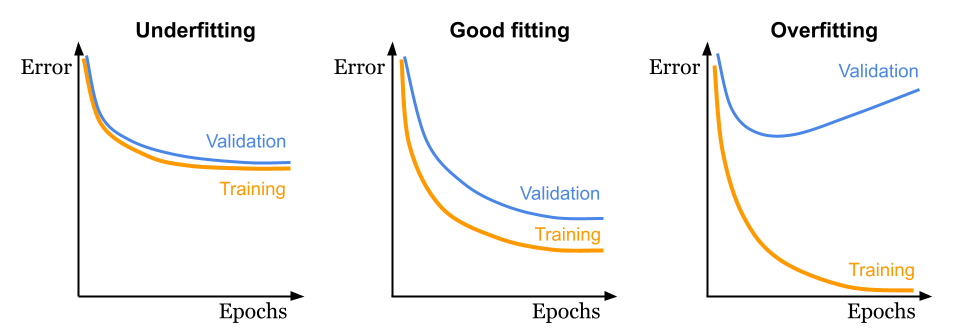
Figure 9.6: Monitoring training and validation losses during model training. The plot illustrates three typical learning behaviours: **underfitting** (both losses remain high and similar), **good fitting** (both losses decrease, with validation loss slightly higher), and **overfitting** (training loss continues to decrease while validation loss plateaus or increases), highlighting the importance of tracking these metrics to assess model performance and generalisation.

Underfitting: The model has been trained with insufficient data or for too few epochs, resulting in similar training and validation losses, which is far from optimal.
Good fitting: Both training and validation losses decrease, with the validation loss slightly higher (worse) than the training loss, which is expected. This represents the ideal scenario.
Overfitting: The model achieves an excellent training loss, but the validation loss does not improve and may in fact diverge. This may indicate overly similar training data or excessive training epochs, preventing the model from generalising to new data.

9.3.6 Fine-Tuning Pre-existing Models

Instead of training a model from scratch, fine-tuning an existing DL model is usually more efficient, especially when your data resembles the dataset used to train the original model. This approach utilises pre-trained weights and previously learned features, significantly decreasing the amount of required annotated data, training time, and computational resources.

9.3.6.1 Applying Transfer Learning

Transfer learning refers to the process of taking a pre-trained model and adapting it to a new but related task by providing task-specific training data, typically in the form of manually annotated image pairs (Figure 9.7). Transfer learning typically involves freezing part of the model (for instance, the initial layers or all layers except the last ones), so their weights are not updated during training. Only the unfrozen layers are updated when the model is trained on new data. Then, the model is trained on the new data, but only the layers that you have unfrozen will be updated. Since the base model already encodes many useful low-level features (e.g., edges, shapes, textures), this approach allows researchers to focus on refining the model for their specific biological structures or imaging modalities^32,33.

This method is especially effective when:

You have limited training data available.
Your imaging conditions closely match those of the pre-trained model.
You wish to quickly adapt a general model to a specific dataset.

9.3.6.2 Conducting fine-tuning

In classic fine-tuning, all layers of the pre-trained model are retrained, with their weights initialised from the original training (Figure 9.7)^15,16. Thus, you continue training the full model using the new data. This approach allows the model to adjust more comprehensively to new data while still preserving the advantages of pre-learned features.

Classic fine-tuning is ideal when:

Your dataset is moderately different from the original training data (e.g., the same biological structure but different staining or modality).
You expect that earlier layers may need to adapt, not just the final classifier or output layers. Early layers in deep networks typically learn to detect general features such as edges, textures, or simple shapes, while later layers capture more complex, task-specific patterns. If your new data differs in basic appearance or imaging modality, updating the early layers helps the model better extract relevant low-level features from your images.
You have enough annotated data to avoid overfitting during full model training. Although this method is more computationally demanding than transfer learning, where only a subset of layers are retrained, it often leads to better results on diverse datasets..

9.3.6.3 Iterative training: keeping humans in the loop

Iterative fine-tuning is an interactive approach that combines model prediction with human annotation (see Section 9.3.4.3). The workflow typically starts with a pre-trained model predicting new images. A user then manually corrects or annotates these predictions, and the improved annotations update the model (Figure 9.7). This cycle continues, progressively enhancing the model’s accuracy with each iteration until it performs as expected^16,34,35.

This method is particularly powerful when:

Annotated data is scarce or expensive to generate.
You work with rare structures, unusual imaging conditions, or new experimental systems.
You want to efficiently build a custom model using feedback from domain experts.

Figure 9.7: Strategies for training DL models for image segmentation. A model can be **trained from scratch** using a large annotated dataset, **fine-tuned** from a pre-trained model with task-specific data, or refined through **human-in-the-loop** workflows where model predictions are manually corrected and fed back for retraining. These approaches balance performance, data availability, and annotation effort.

9.3.7 Evaluating the performance of your model

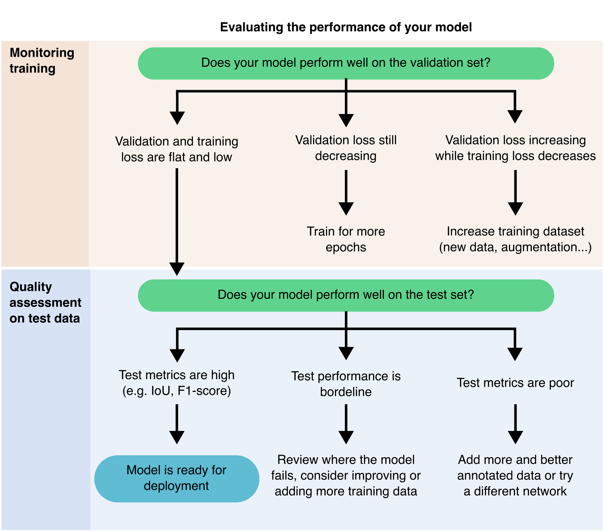
Figure 9.8: Workflow for evaluating DL model performance during training and on test data. Evaluating model performance is essential before deploying any DL model for image segmentation. This diagram outlines a two-stage process: assessment during training and on a separate test set. During training, validation and training losses (see Section 9.3.5.4) guide whether to continue training, stop, or expand the dataset. After training, performance is evaluated using a test set. High test metrics (e.g., IoU, F1-score) indicate readiness for deployment. Borderline or poor results suggest reviewing errors, refining training data, or trying a different model. This approach ensures model reliability and task-specific performance.

With the rapid increase in DL tools and pre-trained models, it has become easier to use DL for image segmentation, but harder to determine which model will work best for your data. Regardless of how promising a model appears, you must always evaluate its performance before trusting its results. Evaluation is not optional; it is a critical step to ensure that the model meets the requirements of your specific task²⁹ (Figure 9.8).

There are two main ways to evaluate a model:

Qualitative evaluation entails visually inspecting the model’s predictions. This approach can help you quickly identify clear errors or failures. It is effective for a small number of images, but it becomes impractical for large datasets or for comparing similar-looking outputs across multiple models.
Quantitative evaluation provides objective metrics for comparing models and tracking improvements. To achieve this, you need a small, labelled test set (typically 5 to 10 images with accurate ground truth segmentations). This test set must remain independent of your training and validation data to ensure an unbiased assessment.

Common metrics used in quantitative evaluation include:

Intersection over Union (IoU), also known as the Jaccard Index, measures the overlap between the predicted segmentation and the ground truth.
F1-score (Dice coefficient): This is especially valuable when the object of interest covers a small area in the image, as it balances precision and recall.
True Positives (TP), False Positives (FP), and False Negatives (FN) are particularly important in semantic segmentation and can be used to calculate the IoU or F1 score.

For more information on these metrics, we recommend²⁹ (also see Chapter 10 for more information).

If a model fails to produce reasonable results, even on simple examples, you can often reject it based solely on qualitative inspection. However, in these cases, quantitative metrics can still help you understand how and where the model fails.

If your evaluation metrics indicate weak performance, especially for certain structures or image types, you may need to fine-tune the model (see Section 9.3.6). Consistently strong scores across various test images suggest that a model could be dependable and ready for deployment. If no pre-trained model meets your expectations, the best course may be to train your model using your images (see Section 9.3.5).

In summary, never skip evaluation. Every model must be tested—both visually and quantitatively—to ensure it truly works for your data and provides results you can trust.

9.3.8 Deploying your model on new data

Once a segmentation model has been trained and validated, it can be used on new, unseen images. This step typically involves feeding new images into the model to generate segmentation predictions. The deployment approach relies on the computational resources (see Section 9.4.2) as well as the size and complexity of your dataset (Figure 9.9).

Figure 9.9: Decision workflow for model deployment strategy based on computational resources. The choice of deployment strategy depends on the availability of computational resources (see Section 9.4.2) and the sensitivity of the data . If high-performance computing resources are available locally, these should be used for deployment. In their absence, consider whether the data can be transferred to the cloud. If so, cloud-based resources offer an efficient solution. However, if data transfer is restricted—due to size or sensitivity—local deployment remains the only option, though it may require significantly more time.

9.3.9 Troubleshooting Common Problems

I found a tool or DL model online, but it does not work. What should I do?

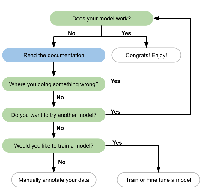
Figure 9.10: Common DL segmentation problems and troubleshooting tips.

When should I train a model or segment manually?

Refer to (Section 9.3.3.2) for more details, but generally, this decision depends on your dataset and the performance of existing pre-trained models (Figure 9.10). If you only need to segment a small number of images, manually segmenting them is often the quickest and simplest solution. However, if you are dealing with a large dataset, it may be more efficient to annotate a small subset and use it to train a deep-learning model that can automate the segmentation of the rest.

I decided to train my DL model, but it is not performing correctly. What should I do?

First, ensure that you have trained the model for a sufficient number of epochs—this depends on the size of your dataset and the architecture of the model. Check the training loss: if it has plateaued, your model may be fully trained. If it is still decreasing, continue training.

If training is completed but results are poor, examine your data. Is the model missing specific features? Are there types of cells or structures that it consistently fails to segment? If so, ensure those examples are well represented and correctly annotated in your training data. You may need to enhance or expand your annotations.

If performance is poor, you may need additional annotated data to help the model generalise more effectively (Figure 9.8). Consider the following questions:

Is my dataset balanced? Does it include sufficient examples of each structure or class I want to segment?
Am I training on one experimental batch while validating or testing on another?

How many images should I have to train my model?

Refer to Section 9.2.1 for more details. There’s no one-size-fits-all answer—it depends on the complexity of your task, your model architecture, and the variability in your data. More complex tasks typically require more data. Larger images can also be broken into more patches, effectively increasing your dataset size. While few-shot models are being developed for small datasets, most established DL models require a substantial amount of data.

Possible technical issues that you may encounter when training your DL model.

The model predicts the same class for all pixels or segments in every cell. Your dataset might be unbalanced, containing too many similar examples. Adding more diverse or underrepresented examples can help the model learn to differentiate between classes.
Out-of-memory errors during training: Consider reducing the batch size or the image patch size. If that doesn’t resolve the issue, consider switching to a workstation or cloud service with greater computational capacity.
The model performs well on training data but poorly on new images, suggesting overfitting (Figure 9.6). Implement data augmentation and increase dataset diversity to help the model generalise better.
Inconsistent results across different computers: Differences in GPUs or environments can cause slight variations in outcomes. If the differences are significant, verify that all systems use consistent software versions and configurations. For further information on this topic, refer to Section 9.4.3.

9.4 Further considerations for DL segmentation

9.4.1 Choosing the Right Tools for DL

Selecting the right tools to train and use DL models depends mainly on your level of programming experience and comfort with technical interfaces.

If you prefer not to write code or use command-line tools, opt for platforms that offer graphical user interfaces (GUIs) or interactive notebooks with pre-configured workflows. These tools let you perform powerful segmentation tasks using intuitive interfaces and simple widgets.

GUI-based tools include, for instance (see Chapter 8 for more tools):

Cellpose GUI
Fiji with DeepImageJ and StarDist plugins
Napari
Ilastik
QuPath

Interactive Jupyter notebooks provide a flexible balance between code and GUI. They enable you to execute code in manageable steps (cells) and immediately see the results. Tools like BiaPy, and DL4MicEverywhere³⁶ leverage Jupyter notebooks, concealing complex code behind user-friendly interfaces. These platforms cater to users with little or no coding experience while still allowing advanced users to access and modify code as needed. DL4MicEverywhere, in particular, established a widely adopted framework for training DL models via notebooks, contributing to the standardisation and simplification of the workflow.

If you are comfortable with programming, you will have even more flexibility. Languages such as Python, MATLAB, Julia, Java, and Rust provide options for building and customizing DL workflows. Python stands out as the most beginner-friendly and widely supported choice, boasting a large ecosystem of libraries and community support. Popular Python libraries for DL include PyTorch, TensorFlow, Keras, and JAX.

While coding can involve a steeper learning curve, it allows you to create customized pipelines, integrate various tools, and troubleshoot intricate workflows, unlocking the full potential of DL for microscopy segmentation.

9.4.2 Managing Computational Resources

When using DL for microscopy, an important consideration is the availability and capacity of your computational resources (Figure 9.9). High-performance DL models, particularly those used for 3D image data, can be very demanding regarding memory and processing power.

When selecting or designing a DL model, evaluate your available infrastructure:

GPU memory: Determines how large your model and batch size can be.
Training time: Influences your ability to iterate quickly; simpler models train faster.
Dataset size: Larger datasets benefit from more powerful hardware and longer training times.

A practical strategy involves starting with lightweight models that demand fewer resources and scaling up to more complex architectures only if performance improvements become necessary. Tools like StarDist and Cellpose, for example, provide efficient options that function effectively with relatively modest hardware.

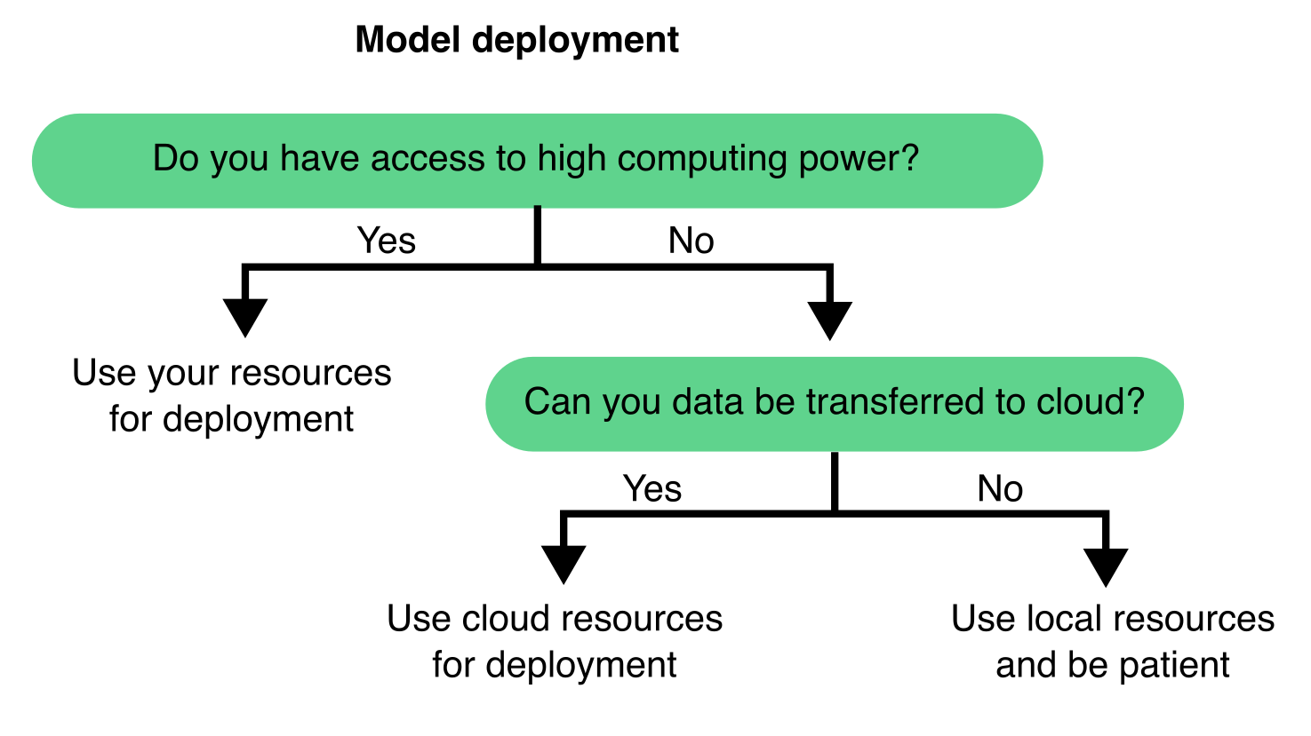
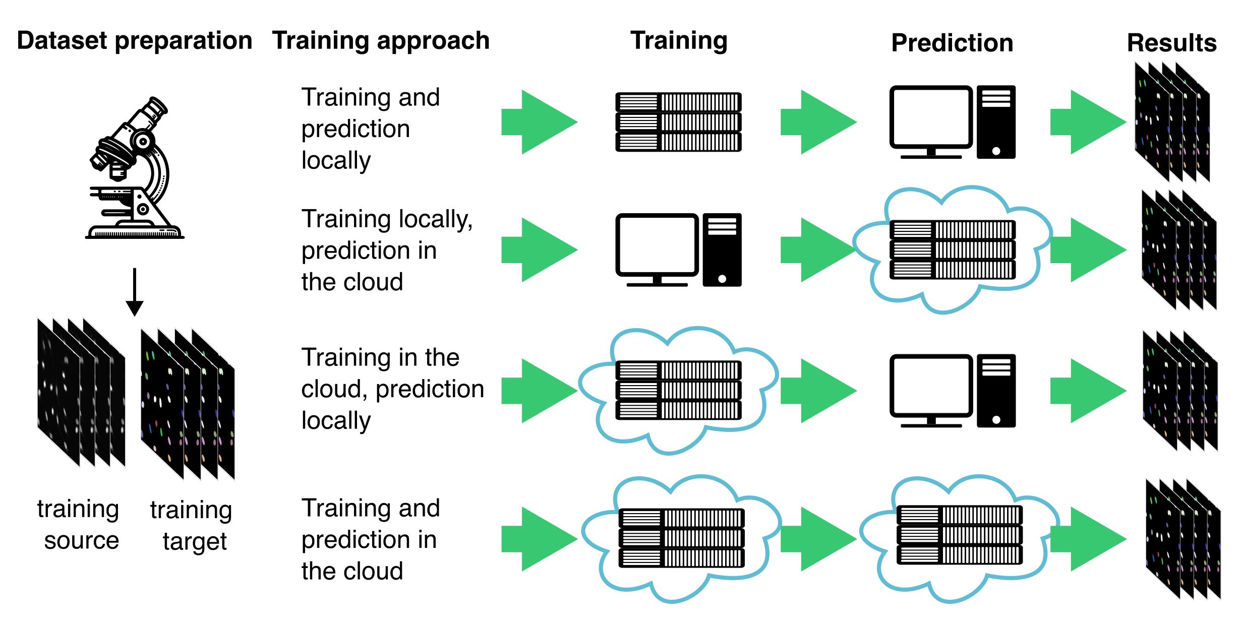
Additionally, consider whether to train and deploy your model locally or in the cloud (Figure 9.11). Local training is often more feasible if you already have access to a compatible workstation and want full control over data and execution. However, cloud-based services like Google Colab or AWS offer access to more powerful hardware, removing the need for local infrastructure—this is especially beneficial when working with large models or 3D datasets.

There are four typical combinations of training and prediction workflows:

Training and prediction locally is well suited for small to medium-sized datasets, especially when computational demands are moderate and data privacy is a priority. This approach also supports some user-friendly desktop applications, such as the Cellpose 2.0¹⁶, which can be run locally without requiring cloud access or advanced technical setup.
Training locally, prediction in the cloud may be useful when models are trained in-house but need to be deployed at scale or integrated into cloud-based pipelines.
Training in the cloud, prediction locally enables researchers to take advantage of powerful cloud GPUs for model development, while keeping inference close to the data source (e.g., a microscope workstation or in case of sensitive data).
Training and prediction in the cloud is well suited for collaborative projects or large-scale deployments, where access to centralized, scalable infrastructure is critical.

Choosing between these strategies depends on your data size, hardware access, choice of software, collaboration needs, and whether your workflow prioritizes flexibility, scalability, or control.

Figure 9.11: Training and deployment strategies for DL models in microscopy. Depending on the available tools and infrastructure, models can be trained and deployed locally or in the cloud. Modified from¹⁷.

9.4.3 Ensuring Reproducibility in DL

When sharing how you trained a DL model, two key elements often come to mind: the dataset used and the code that runs the model. However, in practice, reproducibility extends beyond just data and code. In programming environments like Python, which rely heavily on external libraries, ensuring reproducibility also requires capturing the exact configuration of the environment in which the model was trained.

DL models are sensitive to changes in library versions and dependencies. Even minor differences in the software stack can result in inconsistent outcomes or training failures. While sharing a list of dependencies (e.g., a requirements.txt or a Conda environment file) is a constructive step, differences in operating systems or local setups can still lead to issues.

A robust and increasingly popular solution is containerisation. Containers package software, dependencies, and environment settings into a portable and self-contained unit. One of the most widely used containerization tools is Docker. A Docker container can be considered a lightweight, standalone virtual machine that includes everything needed to run code, such as the operating system, libraries, and runtime, ensuring applications run consistently across different machines.

Using containers ensures that your model training and inference processes remain consistent, no matter who executes them or where they are conducted. This greatly simplifies the ability of collaborators or reviewers to reproduce your results.

For researchers unfamiliar with software development, tools like DL4MicEverywhere³⁶ and bia-binder³⁷ simplify the use of containers by integrating them into user-friendly Jupyter notebook environments. These platforms enable researchers to benefit from the reproducibility of containers without needing to manage complex setups or command-line tools.

Reproducibility is crucial for establishing trust in computational results and facilitating long-term scientific collaboration. To ensure your DL workflows are reproducible, follow these best practices:

Pin every software version used in your workflow.
Document your environment setup thoroughly.
Provide a containerised version of your training and inference pipeline when possible.
Taking these steps will make it easier for others to reproduce your results, build on your work, and apply your models in different research settings.

For more information on best practices, consult²⁹.

9.5 Summary & Outlook

Segmenting microscopy images remains a critical yet challenging task in bioimage analysis. In this chapter, we have used segmentation as a representative example to illustrate deep learning workflows and considerations. However, the strategies and best practices described here—such as data preparation, model selection, training, evaluation, and deployment—are relevant to a wide range of image analysis tasks, including classification, detection, and tracking. DL has undeniably transformed this field, offering robust solutions for segmenting complex and variable structures. However, as this chapter emphasizes, DL is not always the fastest or the best approach. Classical image processing techniques or pixel classifiers often provide faster, simpler, and highly effective alternatives in many scenarios.

The decision to use DL should be driven by the complexity of the task, the availability of annotated data, and the specific goals of the segmentation project. Successful DL implementations often require significant investments in data curation, annotation, and computational resources. Furthermore, training from scratch is frequently avoidable thanks to the growing ecosystem of pre-trained models and resources shared by the community.

Notably, the landscape of DL segmentation is rapidly evolving. The emergence of foundation models, which are large, versatile networks pre-trained on vast and diverse datasets, promises to further lower the barriers to entry¹⁵. These models enable transfer learning, fine-tuning, and even zero-shot segmentation, where accurate predictions can be made on previously unseen data with minimal or no task-specific training. This shift opens exciting new avenues for researchers who previously lacked the resources or expertise to apply DL in their work.

The ongoing development and democratization of DL tools, along with enhancements in model generalisability, human-in-the-loop workflows, and reproducibility, are changing how microscopy data is analyzed. Still, the key to successful segmentation will always involve careful planning, quality control, and selecting the right tool for the task, whether it involves DL or not.