6  Image Restoration

Using Artificial Intelligence for Image Restoration in Fluorescence Microscopy

Authors

Affiliations

Yue Li

Zhejiang University

Jun Zhu

Zhejiang University

Mingzhe Wei

Zhejiang University

Hari Shroff

HHMI Janelia Research Campus

Min Guo

Zhejiang University

Fluorescence microscopy is central to biological discovery, enabling the visualization of cellular and subcellular structures with exquisite detail. From observing dynamic intracellular processes to mapping entire tissues, microscopy is indispensable for understanding biological systems¹. However, the quality of microscopic images is often compromised due to intrinsic limitations such as noise, optical aberrations, diffraction, and limited signal². These factors hinder analysis and interpretation, particularly when studying fine biological structures or dynamic processes. For example, by quantifying the intensity of fluorescence signals, researchers infer the abundance or expression levels of specific molecules (e.g. proteins tagged with a genetically expressed marker). Using image segmentation, researchers can analyze the size, shape, distribution and number of specific objects within a defined region³. By tracking the movement of fluorescently labeled molecules or cells over time, researchers can study processes including endocytosis, intracellular transport, and cellular signaling⁴. In these scenarios, noise and low SNR can make it difficult to distinguish between the actual signal and background; and spatial blurring causes fluorescence signal to spread out, confounding the ability to accurately assign pixels to specific regions or structures.

Many of these problems can be overcome with suitable hardware or by using advanced imaging techniques. To improve spatial resolution, super-resolution techniques (stimulated emission depletion (STED), structured illumination microscopy (SIM), or single-molecule localization microscopy (SMLM)) may be employed⁵. To suppress noise and maximize the collection of useful signal, highly sensitive detectors, such as cooled charge-coupled devices (CCDs) or complementary metal-oxide-semiconductor (CMOS) sensors can be used. To correct optical distortions, advanced microscopes integrate adaptive optics (AO)^6,7, which use real-time feedback to dynamically adjust the focus and compensate for aberrations. However, these technologies often come with high cost, require complex operation, or need extensive maintenance. Additionally, improving one attribute of the image (e.g. spatial resolution) often results in a compromise in another (e.g., temporal resolution), requiring careful consideration of the specific needs of a study and the resources available⁸.

Another way to address these limitations is to develop image restoration techniques that enhance the quality of microscopic images, often without expensive instrumentation. Traditionally, these techniques relied on mathematical algorithms and physical models of the imaging process. However, recent advances in artificial intelligence (AI), particularly deep learning, have transformed image restoration by enabling data-driven approaches that offer improved performance and flexibility. Manufacturers have increasingly integrated image restoration technologies as an essential component of their products to ensure their users can obtain clearer images directly from the microscope, e.g., Leica THUNDER Imager, Olympus cellSens, Andor iQ, ZEISS arivis, and Nikon NIS-Elements.

In this chapter, we provide a practical overview of image restoration for applications in fluorescence microscopy. We begin by introducing the general concept of image restoration, then describe traditional and deep learning-based approaches. Next, we review key technologies and advances by categorizing restoration into four major areas: denoising, deconvolution, deaberration, and resolution enhancement. Finally, we provide practical guidelines for implementing image restoration, including step-by-step workflows and test datasets for interested readers to practice applying these methods.

6.1 General Concepts in Image Restoration

Image restoration is the application of mathematical and computational techniques aimed at improving the quality of an image by reversing or reducing the effects of degradation that may occur during the imaging process. These degradations stem from noise, blur, aberrations, and other artifacts. The goal of the restoration is to recover or estimate the latent (true) image from the degraded raw data. Image restoration has the potential not only to improve the precision of biological analyses but also to expand the capabilities of existing microscopes, enabling researchers using basic hardware to achieve advanced imaging quality.

6.1.1 Image Degradation Model

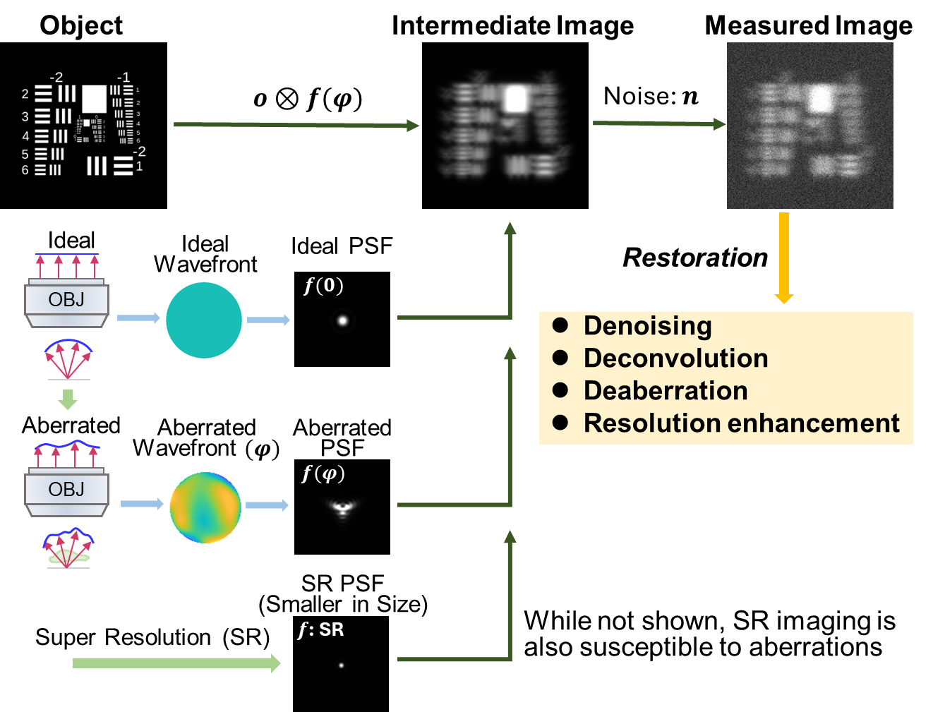
Understanding the types of distortions and the causes behind them is the first step in image restoration. This could involve a mathematical model that characterizes how an image is corrupted, using the concept that any real-world imaging system cannot capture an object perfectly. Instead, the imaging system or sample introduces imperfections, which distort the image. In fluorescence microscopy, a general image degradation model can be written as:

\[ i = o \otimes f ( \phi ) + n \tag{6.1}\]

Where \(i\) is the image acquired by the microscope; \(o\) is the intensity distribution of the biological sample; \(f(\phi)\) is the point spread function (PSF) of the system; \(\phi\) is the phase aberration or wavefront distortion (when \(\phi=0\), the wavefront is ‘flat’ or aberration-free and \(f\) is the ideal PSF predicted by theory); \(\bigotimes\) is the convolution operator; and \(n\) models noise contamination. Two common types of noise are Gaussian noise and Poisson noise. Gaussian noise is caused by random fluctuations in the image due to imperfections in the camera sensor or electronic interference. Poisson noise arises from the random nature of photon detection, meaning that the number of photons detected can vary from one measurement to the next, especially at low light levels. Equation 6.1 is described schematically in Figure 6.1.

Figure 6.1: Schematic of image degradation model for fluorescence microscopy. Object information passes through the imaging system with degradation due to blurring from the point spread function (PSF, here denoted by the convolution kernel \(f\)) and noise. In an ideal case, there is no distortion, and the wavefront associated with a point source maintains a flat phase at the back focal plane of the microscope objective. In any real situation, wavefront distortion due to optical imperfections or heterogeneity within the biological sample results in an aberrated wavefront (indicated by \(\phi\)) and PSF, which results in additional blurring. If spatial resolution is enhanced, e.g., by super-resolution methods (SR), the PSF becomes smaller, resulting in sharper images. Super-resolution imaging is also (typically more) prone to aberrations than conventional diffraction-limited imaging, and noise is inherent to any imaging process.

6.1.2 Image Restoration with Traditional Approaches

Traditional microscopy image restoration techniques use mathematical modeling of the imaging model and statistical analyses that attempt to reverse or mitigate image degradations, and/or additional microscope hardware. We find it helpful to categorize image restoration into four main areas: denoising, deconvolution, deaberration, and resolution enhancement.

6.1.2.1 Denoising

Traditional denoising methods try to remove noise while preserving important features such as edges and fine structures. Many denoising algorithms assume Gaussian noise, for computational tractability. Gaussian noise removal can be achieved by filtering-based methods in the spatial or frequency domain, such as Gaussian filtering, mean filtering, wavelet filtering, bilateral filtering⁹, and non-local-based BM3D¹⁰. Simple linear filters are easy to implement, but they cause a loss in high-frequency information. Complex denoising methods require careful parameter design and are usually computationally intensive. In many cases, the Gaussian noise model provides a good approximation, but Poisson noise is also a key source of noise for fluorescence microscopy given the quantized nature of fluorescence emission, especially under low signal conditions when detector noise is minimal. One method for dealing with Poisson noise¹¹ directly incorporates its statistics, e.g. the PURE-LET method¹². Alternatively, a nonlinear variance-stabilizing transformation (VST)¹³ can be used to convert the Poisson denoising problem into a Gaussian denoising problem. There are several free and open-source resources available for microscopy image denoising, including filters and the PureDeNoise¹⁴ plugin in ImageJ/Fiji, and the scikit-image library in Python¹⁵.

6.1.2.2 Deconvolution

Deconvolution is the process of reversing optical blur introduced by the PSF of the microscope (\(f(\phi)\) in Figure 6.1) and is most often implemented without considering optical aberrations. It improves effective contrast and resolution by accounting for such blur and reassigning the relevant signal to its most likely location, given the blurring and noise models. Traditional deconvolution methods include frequency-domain algorithms like naive inverse filtering and Wiener filtering^16,17, optimization-based algorithms like Tikhonov regularization¹⁸, and iterative deconvolution methods like the Tikhonov-Miller algorithm¹⁹, fast iterative soft-thresholding algorithm²⁰, and Richardson-Lucy deconvolution^21,22. Traditional deconvolution methods can require significant computational resources, especially for large datasets with complex blurring functions, and also can amplify noise^23–25. Commercial deconvolution software includes Huygens, DeltaVison Deconvolution, and AutoQuant. There are also open-source deconvolution plugins integrated into Fiji²⁶ (e.g., DeconvolutionLab2²⁷) or MIPAV²⁸ (Medical Image Processing, Analysis, and Visualization, https://mipav.cit.nih.gov/) programs.

6.1.2.3 Deaberration

Aberrations refer to the optical imperfections or distortions that occur during image acquisition, degrading the quality of the captured image. Such aberrations can arise due to optical path length differences introduced anywhere in the imaging path, including instrument misalignment, optical imperfections, or differences in refractive index between the heterogeneous and refractile sample, immersion media, and/or objective immersion oil. Aberrations significantly alter the wavefront of light. When the wavefront is distorted, the light rays that are focused by the microscope do not converge as they ideally should. This distortion can lead to various image quality issues, such as loss of resolution, and distortion of fine features. Adaptive optics^6,29 can mitigate aberrations by measuring wavefront distortions and subsequently compensating for them using a deformable mirror or other optical elements. However, implementing AO is nontrivial, often requiring additional control algorithms and new hardware, adding considerable expense to the underlying microscope.

6.1.2.4 Resolution Enhancement

Optical super-resolution techniques, like STED, PALM, SIM, etc., bypass the diffraction limit by utilizing on/off fluorophore state transitions³⁰, sophisticated hardware designs, and/or image reconstruction algorithms^4,31,32. Alternatively, physical expansion of the sample can be used with conventional microscopes^33,34. While effective, all these methods present some tradeoff for the gain in spatial resolution, including increased acquisition time, additional illumination dose, specially designed probes, or more complex instrumentation^35,36.

6.1.2.5 Drawbacks

Although traditional image restoration algorithms are used extensively in all these categories, they suffer several drawbacks. For example, many methods require careful and manual parameter tuning, and they often perform poorly in challenging conditions, such as in the presence of high noise, low contrast, defocus, or complex background. This is often because they are based on idealized assumptions (Equation 6.1), which are often not met in practice. Another limitation of traditional restoration methods is that they are generally ‘content unaware’ and do not use sample-specific prior information (e.g., shape, size, intensity distributions). On the one hand, this means that traditional algorithms generalize well, but on the other hand, they are not as performant as newer deep learning methods. Deep learning methods can learn a task such as denoising from the data themselves or provide a sample-specific prior³⁷, and thus can outperform traditional methods in many cases.

6.1.3 Image Restoration with Deep Learning-Based Approaches

Artificial intelligence (AI), particularly deep learning, has achieved remarkable progress in recent years, leading to breakthroughs in image restoration tasks. Deep learning uses artificial neural networks with multiple layers to model and learn complex patterns in data through end-to-end training, eliminating the need for handcrafted features or manual parameter tuning. By leveraging large datasets and computational power, deep learning can capture non-linear relationships and subtle details within image data, making it particularly well-suited for image restoration. Techniques such as convolutional neural networks (CNNs), generative adversarial networks (GANs), autoencoders, and transfer learning have been shown to tackle applications in denoising, deblurring, super-resolution, and deaberration. Recent advances, such as content-aware restoration (CARE)³⁸, residual channel attention networks (RCANs)³⁹, and deep Fourier-based models⁴⁰, have demonstrated improvements in image quality while reducing phototoxicity and photobleaching during acquisition. These models offer several advantages over more traditional methods of image restoration:

• Automatic Feature Learning: Traditional image restoration methods rely heavily on manually designed features (e.g., regularization selection) and parameter tuning, which often require fine adjustments for different types of images. Deep learning models, on the other hand, can automatically learn features from large datasets, eliminating the need for manual intervention. This significantly reduces the complexity of parameter tuning and makes the models more adaptable to complex samples or tasks.

• Strong Non-Linear Modeling Capabilities: Traditional algorithms are often based on linear image degradation models (Equation 6.1), which ignore sample-specific information and perform poorly in the presence of complex image distortions or noise. However, recovering the object structure from the acquired image is an inherently ill-posed and nonlinear problem due to noise and blurring. Deep learning uses nonlinear activation functions (ReLU, sigmoid) and hierarchical layers to approximate complex relationships in the image data. Thus, deep learning can better model the global context of an image, allowing for more accurate restoration of image details under challenging and suboptimal imaging conditions. This can extend the use of existing hardware beyond its original use to new biological questions that were previously inaccessible.

• Efficient Handling of Complex Scenes: Deep learning models are typically trained on large datasets and are capable of handling complex scenes (e.g., images contaminated with noise and aberrations⁴¹) and large-scale data (e.g., GB- or TB-scale time-lapse data). Once a model is trained, it can automatically adapt to new input data with similar acquisition parameters, which makes it much more efficient for large-scale image restoration tasks.

As deep learning models continue to evolve and integrate with advanced microscopy hardware and large datasets, they are expected to further push the boundaries of biological imaging and discovery. In the next section, we will introduce the application of deep learning methods in different image restoration tasks.

6.2 Deep Learning-Based Techniques for Image Restoration

Following the convention from Section 6.1.2, we group AI-based restoration into four broad categories.

6.2.1 Denoising

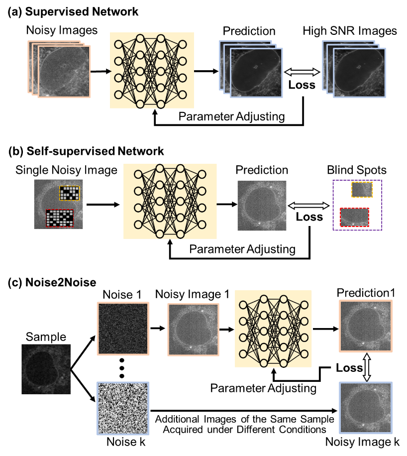
Traditional denoising techniques struggle to preserve fine details while removing noise^40,42,43. Deep learning-based methods, on the other hand, can learn to predict what fine details look like even in the presence of noise. Such methods can be generally divided into supervised learning and self-supervised learning (Figure 6.2). Supervised learning methods require a large number of paired datasets of noisy and clean images for training. These datasets can be obtained by tuning illumination intensity and/or exposure time during image acquisition: when imaging with high intensity or longer exposure time, high-SNR clean images can be collected; otherwise, noisy images are collected. Training a supervised deep learning method on these data results in a mapping between noisy and clean images. When sufficient training data is available, these methods can provide very high-quality restoration on noisy data unseen by the network in the training process. However, paired datasets can be difficult to obtain in some microscopy settings (e.g., live-cell imaging). Typical denoising networks include U-Net-based Content-aware image restoration (CARE)³⁸ and attention-based residual channel attention networks (RCAN)³⁹.

Self-supervised learning methods do not require paired noisy and clean images. Instead, only noisy images are needed for training. They exploit the inherent structure of the data, learning to predict parts of the image using information gleaned from other parts. Typical self-supervised methods include Noise2Void (N2V)⁴⁴ and Noise2Self (N2S)⁴⁵. The key idea underlying N2V and N2S is that pixels from clean images are often highly correlated, i.e., nearby pixels usually look similar and follow predictable patterns. For example, neighboring pixels could show smooth gradients in image texture. However, many noise sources are are randomly correlated in space, particularly across large areas. So by selecting a suitable mechanism, noise and signal can be separated properly. In N2V, missing pixels are randomly masked in the noisy input image and the network is then trained to predict the value of the missing pixel using the surrounding noisy pixels. In N2S, instead of masking the noisy image entirely, local patches are used, and the network is trained to predict the value of the noisy pixel from its neighbors. While self-supervised methods can be effective, they often do not perform as well as supervised methods when the sample or noise distribution is complex. These methods nevertheless are quite useful when paired noisy-clean images are difficult or impossible to obtain.

Noise2Noise (N2N)⁴⁶ represents another kind of supervised training. It trains the model using two noisy images (A and B), where both images contain the same underlying clean signal. Essentially, it learns to map noisy image A to noisy image B. Since both images share the same clean signal beneath the noise, the network can learn to recover the underlying clean image. This method still relies on paired data as supervision, but the supervision signal comes from another noisy image rather than a traditional clean image.

Figure 6.2: Different denoising methods for microscopy images. (a) Supervised denoising methods^38,39, train a neural network using paired noisy and high-SNR images. (b) In self-supervised methods^44,45, a portion of the image is masked (blind spots or black pixels in yellow and red subregions) for training, removing the need for explicit high-SNR images. (c) The Noise2Noise network⁴⁶ is another form of supervised training, whereby the network is trained with a set of noisy images of the same underlying sample.

6.2.2 Deconvolution

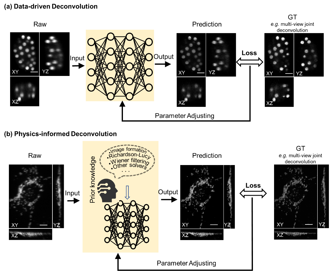
Deconvolution has long relied on iterative algorithms like the Richardson-Lucy method. Recent advances in deep learning (DL) have revolutionized this task, offering high speed and in some cases even more accurate predictions than traditional methods⁴⁷. Deep learning deconvolution methods can be divided into two categories: purely data-driven learning and physics-informed learning (Figure 6.3).

In the data-driven approach, training is conducted similarly to supervised denoising methods. The raw images are the low-quality blurred acquisitions; the high-quality reference can be the results of traditional restoration (e.g., multi-view jointly deconvolved results, or high SNR deconvolved results). Models like CARE, RCAN, and DenseDeconNet²⁵ can be used for deconvolution. Once trained, such data-driven deconvolution generally enables more rapid deconvolution than traditional methods. However, these methods are content-aware and depend heavily on high-quality paired training data. This criterion may introduce artifacts and affect how well the network generalizes.

Physics-informed methods integrate domain knowledge—such as the microscope’s point spread function (PSF), and image formation models—into the network architecture or loss functions. For example, the Richardson-Lucy Network (RLN)⁴⁷ embeds Richardson-Lucy iterations within a convolutional network, creating a hybrid method that leverages classical knowledge and data-driven deep learning. MultiWienerNet uses multiple differentiable Wiener filters paired with a convolutional neural network, exploiting the knowledge of the system’s spatially varying PSF to quickly perform 2D and 3D reconstruction, achieving good results on spatially varying deconvolution tasks⁴⁸. Physics-informed methods can also improve interpretability and reliability and may reduce the demand for experimental training data by leveraging synthetic data generated from optical models.

Figure 6.3: Different Deep Learning-Based Methods for Deconvolution in Microscopy Images. (a) Data-driven based deconvolution methods^25,38, where a neural network is trained using only a large-set of paired raw data and ground truth (GT, e.g., joint deconvolution of multiview data) . (b) Physics-informed deconvolution^47,48, whereby a neural network is trained using not only paired datasets but also incorporatesprior physical knowledge, such as embedding the image formation function in the loss function and/or the Richardson-Lucy framework or Wiener filtering in the network architecture.

6.2.3 Deaberration

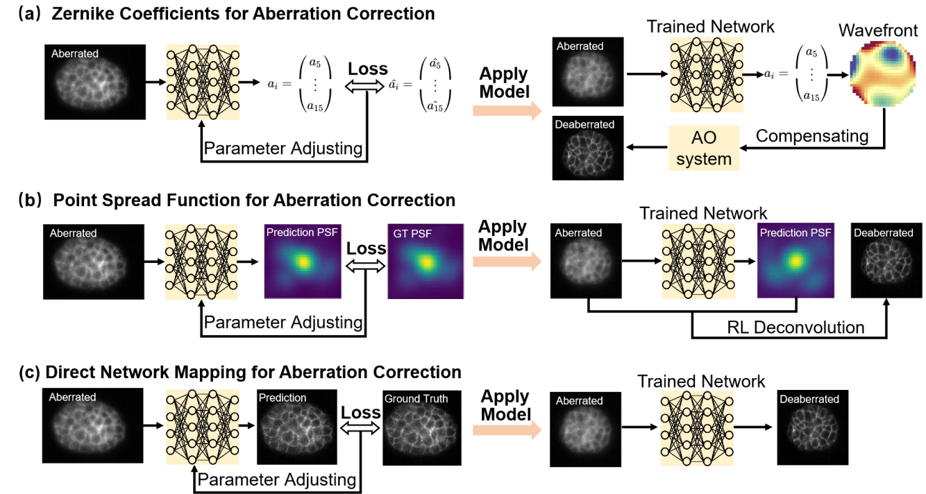
Deaberration addresses image degradation caused by optical distortions due to refractive index mismatches in biological samples or imperfections in the optical system. These aberrations degrade image quality, particularly in thick or scattering samples. Recent advances in deep learning have introduced powerful alternatives to traditional AO for both explicit wavefront estimation and the prediction of cleaner images in which aberrations are suppressed (Figure 6.4).

Initial efforts focused on estimating the distorted wavefronts with AI, followed by explicit wavefront correction with hardware (e.g., a deformable mirror, or SLM) to obtain a clean image. The wavefront aberration can be decomposed as a sum of Zernike polynomials. The problem of wavefront estimation then becomes inferring the amplitudes of different Zernike polynomials⁴⁹. This approach combines the strengths of traditional AO with artificial intelligence^50–52. Following the concept of deconvolution, researchers have also used deep learning to predict the aberrated wavefronts or blurring kernels (aberrated PSFs), also combining this information with post-processing deconvolution algorithms for image restoration^53,54.

In contrast to explicit wavefront prediction, other efforts have trained neural networks directly on paired aberrated and corrected images^55,56. These models are designed to learn the mapping between aberrated and corrected images, enabling aberration correction as a purely computational post-processing step. This approach eliminates the need for hardware-based wavefront sensing or correction, making it a practical and scalable solution for many microscopy applications. More recently, a unified deep learning framework for simultaneous denoising and deaberration in fluorescence microscopy has also been developed⁴¹. By addressing both noise and aberrations in a single model, this approach simplifies the image restoration pipeline while delivering high-quality results, highlighting the potential of multitask models to streamline microscopy workflows.

Figure 6.4: Different Deep Learning-Based Methods for Aberration Correction in Microscopy Images. (a) A method where the network is configured to learn the distorted wavefront (using a sparse representation of Zernike coefficients)^50–52. The trained network is then used to predict wavefront distortions (in terms of Zernike coefficients) for a new dataset, followed by hardware-based correction using an adaptive optics (AO) system (e.g., a deformable mirror). (b) A method where the network is configured to learn the aberrated Point Spread Function (PSF)^53,54. The trained network is then used to predict the aberrated PSF corresponding to a new dataset, and a second step of image deconvolution is applied with the predicted PSF to remove aberrations from raw images. (c) A method where a neural network learns the mapping between aberrated and corrected images directly for post-processing aberration correction^55,56. The trained network is then used to directly predict the deaberrated image corresponding to a new dataset.

6.2.4 Resolution Enhancement

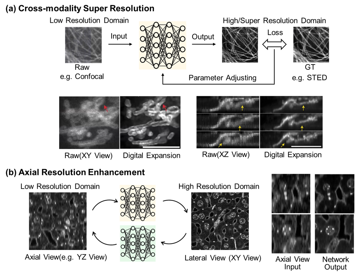
The spatial resolution of optical microscopy is fundamentally limited by the diffraction of light, a barrier described by Abbe’s law. Deep learning methods can learn to predict what a higher resolution image might look like, given lower resolution input data (Figure 6.5). Such methods use artificial neural networks to infer high-resolution (HR) details from low-resolution (LR) fluorescence images, which can offer a sharper image without the need for super-resolution microscopes. Cross-modality super-resolution (CMSR) refers to a class of techniques that use information from different imaging modalities to enhance resolution. Models such as CNNs and GANs are trained to learn the mapping between these modalities. For example, researchers can use super-resolution (e.g., STED) images to enhance diffraction-limited (e.g., confocal) images⁵⁷; or use models trained on expansion microscopy data to predict super-resolution images from diffraction-limited inputs. Fourier-based approaches (e.g. DFCAN⁴⁰) leverage the frequency content difference across distinct features in the Fourier domain to enable the networks to learn the hierarchical representations of high-frequency information efficiently. While powerful, we note that these resolution enhancement methods offer a prediction at best and cannot truly retrieve higher resolution information absent in the low-resolution input data.

Another resolution enhancement task is the prediction of isotropic resolution from blurry axial views. The majority of fluorescence microscopy techniques, including most widefield, confocal, and light-sheet microscopes, suffer from unmatched resolution in the lateral and axial directions (i.e., resolution anisotropy), which severely deteriorates the quality, reconstruction, and analysis of 3D images. Deep learning models can be trained to predict and fill in the missing information in the z-direction using the higher lateral resolution view and knowledge of the anisotropic PSF, effectively making the resolution more uniform across the entire image^58,59.

Figure 6.5: Schematic of resolution enhancement with cross-domain networks. (a) Cross-modality super resolution^39,57. Top row: the method takes diffraction-limited data (e.g., confocal microscopy data) as input and super-resolved data (e.g., STED microscopy data or expansion microscopy data) as ground truth. By training a neural network with paired datasets, the network parameters are updated based on the loss between the network’s output and the ground truth, thereby achieving a mapping from the low-resolution domain to the high-resolution domain. Bottom row: similar cross-modality learning can also be adapted using expansion microscopy as the ground truth. The red and yellow arrows highlight improvements in lateral and axial slices due to the restoration process. By ‘digital expansion’, we mean the super-resolution prediction based on expansion microscopy ground truth. (b) Axial resolution enhancement^58,59. The method uses datasets composed of low-resolution axial slices (sometimes synthesized from higher resolution lateral views³⁸) and high-resolution lateral slices, employing a one-step⁵⁸ or two-step⁵⁹ framework to learn the mapping from the low-resolution domain to the high-resolution domain, thus achieving axial resolution enhancement for fluorescence microscopy 3D stack data.

6.3 Practical Guidelines for Image Restoration

For researchers new to deep learning-based image restoration, successfully applying deep learning to image restoration requires careful preparation and a clear understanding of basic concepts. Here we briefly describe practical guidelines to help you get started with using deep learning for image restoration, from data preparation to model deployment. A step-by-step manual for different image restoration tasks (i.e., denoising, deconvolution, deaberration, and resolution enhancement) using RCAN is provided in Appendix A.

6.3.1 Considerations for Dataset Preparation

Microscope Compatibility: Ensure images are captured with consistent settings (e.g., exposure time, magnification). Common sources include confocal, widefield, light-sheet, or super-resolution microscopes.

Paired vs. Unpaired Data: Paired data (low-quality – high-quality pairs) is ideal for supervised learning. Acquire paired datasets of degraded and high-quality images for supervised training. In contrast, unpaired data is typically used for for self-supervised methods (e.g., Noise2Noise). For unsupervised methods, collecting degraded images with varying conditions (e.g, different noise levels) helps the model generalize better across different conditions.

Training Data Size: According to the size of the acquired data, start with at least dozens of datasets of size 128×128 for 2D and 128×128×128 for 3D. Augmentation with rotations, flips, and noise injections can expand your training dataset (see also Chapter 5).

6.3.2 Choosing a Network Architecture

The choice of network architecture can play an important role when performing image restoration (see also Chapter 4). Here are some popular architectures used for this purpose:

• Convolutional Neural Networks (CNNs): CNNs are currently commonly used because they are highly effective at capturing spatial features in images. For example, you can use U-Net⁶⁰, a popular CNN architecture designed for image segmentation that is also well-suited for restoration tasks.

• Generative Adversarial Networks (GANs): GANs can be used for tasks like image generation or synthesis (e.g., resolution enhancement), where the goal is to generate realistic images from degraded inputs. GANs consist of two networks: a generator (which creates images) and a discriminator (which evaluates the quality of the generated images).

• Autoencoders: These are unsupervised learning models that can be used for denoising, inpainting, and compression. Autoencoders consist of an encoder and a decoder that map input data into a lower-dimensional representation and then reconstruct it.

• Choose or design networks (e.g., CARE, Noise2Void), or even start with pre-trained models for faster deployment.

6.3.3 Training

Once you have your data, hardware, and software environment and have chosen a model architecture, it’s time to train the model (see also Chapter 9). Training involves feeding the model the degraded images and their corresponding high-quality ground truth and then updating the model weights to minimize the difference between the restored and the ground truth images.

Loss Functions: Common loss functions for image restoration include mean squared error (MSE), structural similarity index (SSIM), and perceptual loss, which helps preserve perceptually important image details.

Optimization: Use optimizers like Adam or SGD (Stochastic Gradient Descent) to update the model’s parameters during training.

Training deep learning models can take a significant amount of time, depending on the size of the dataset, the complexity of the model, and the hardware you use. You can use techniques like early stopping⁶¹ to avoid overfitting and ensure the model is trained for an optimal number of epochs^62,63.

6.3.4 Validation and Deployment

After training, it’s important to evaluate your model’s performance (see also Chapter 10). This can be done by testing it on a separate validation set (with ground truth reference) or test set (without ground truth) that wasn’t used during training.

Common evaluation metrics for image restoration include peak signal-to-noise ratio (PSNR), SSIM, and Visual Quality Assessment. These metrics help assess how close the restored images are to the ground truth in terms of quality and structure. Perform biological validation to ensure restored images are artifact-free, such as expert evaluation, cross-validation with alternative techniques, or repeat experiments to evaluate uncertainty.

If the initial results are not satisfactory, you may need to fine-tune your model. This can involve: adjusting the model architecture (e.g., adding more layers or changing the number of filters); using a different loss function; and fine-tuning hyperparameters like the learning rate.

Once your model has been trained and evaluated, the next step is deploying it. Depending on the use case, you might deploy it for real-time image restoration or integrate it into a larger image processing pipeline.

6.4 Limitations and Future Perspectives

The integration of artificial intelligence (AI) into fluorescence microscopy image restoration has opened new avenues for biological discovery. However, as the field evolves, critical challenges and opportunities must be navigated carefully. Below, we outline key failure modes, caveats, and emerging trends, including the role of transformers and large models, to guide future research.

6.4.1 Caveats of AI-based image restoration

While AI has made remarkable strides in fluorescence image restoration, there are still failure modes that researchers must be aware of. One potential issue is overfitting, where a model becomes too specialized to the training data and struggles to generalize to unseen data. This can result in poor restoration performance on images that differ from the dataset used for training.

Additionally, loss of fine details^40,64 and artifact generation^11,65 remain a concern. Restored images may exhibit blurring, distorted textures, or unrealistic artifacts⁶⁶, especially in high-resolution regions or when attempting to restore challenging image regions (e.g., dense and overlapping structures⁶⁷ or highly degraded structures⁴¹). For example, while doing confocal-to-STED microscopy restoration with RCAN, certain microtubules evident in the STED remain unresolved in the RCAN result, and RCAN prediction for nuclear pores revealed slight differences in pore placement relative to STED ground truth³⁹. While denoising fly wing data with CARE, the same networks predicted obviously dissimilar solutions across multiple trained models³⁸. During denoising, conflicts between restoring local details and enhancing global smoothing can arise^68,69. Due to AI’s inability to achieve a global understanding of semantic information, stitching artifacts may arise during large-scale data processing involving tiling operations⁷⁰, resulting in inconsistent intensity, geometry, and textures. These artifacts may not always be immediately noticeable but can significantly affect subsequent analysis and interpretation. Ensuring algorithm robustness across varied datasets and imaging conditions is key to minimizing these issues.

Deep learning models often operate in a “black-box” manner. This means that while these models can produce useful predictions, the reasoning behind their predictions is not easily interpretable by humans. This lack of transparency and interpretability means researchers might not know exactly how or why certain features in an image are being restored in specific ways. This issue can undermine trust in the model’s results and limit its acceptance in critical applications.

AI-based image restoration techniques are highly dependent on the quality of training data. For fluorescence images, obtaining high-quality ground truth data can be challenging, especially when using highly specific imaging conditions or performing imaging on rare biological samples. The availability and variability of the resulting data can limit the model’s ability to generalize to diverse datasets.

Deep learning models can be computationally expensive during training and require powerful hardware for training and inference. This can be a significant barrier for some research labs or organizations with limited access to high-performance computing resources. Researchers need to consider these limitations when planning AI-based restoration projects and balance trade-offs between model complexity, data availability, and computational requirements.

6.4.2 Outlook for the Future

With advances in transfer learning and self-supervised learning, AI models are likely to become more efficient, requiring less annotated data and computational power. As datasets grow and become more diverse, the dependency on highly specialized ground truth data will be reduced. Moreover, the integration of AI with microscopy platforms in real-time will enhance the ability to process images on the fly, providing immediate feedback to researchers and enabling dynamic imaging of live cells and tissues.

Newer methods of AI will be developed. Transformer models and large-scale models have shown remarkable success in other domains like natural language processing and computer vision. Transformer architectures, known for their ability to capture long-range dependencies and global context, could significantly improve image restoration tasks by better handling complex, large-scale image structures. Large models—trained on massive datasets—are likely to offer even greater performance, able to generalize across different imaging modalities and restoration tasks. As computational resources continue to expand and more sophisticated models are developed, we can expect these methods to further push the boundaries of image restoration, achieving even finer levels of detail and more accurate reconstruction.

In conclusion, the future of AI in fluorescence microscopic image restoration is bright. While challenges such as interpretability, data quality, overfitting, and computational demands remain, the field is poised for rapid advances with new architectures and training techniques.

1.

Wu, Y. & Shroff, H. Multiscale fluorescence imaging of living samples. Histochemistry and Cell Biology 158, 301–323 (2022).

2.

Schermelleh, L., Heintzmann, R. & Leonhardt, H. A guide to super-resolution fluorescence microscopy. Journal of Cell Biology 190, 165–175 (2010).

3.

Archit, A. et al. Segment anything for microscopy. Nature Methods 22, 579–591 (2025).

4.

Sahl, S. J., Hell, S. W. & Jakobs, S. Fluorescence nanoscopy in cell biology. Nature Reviews Molecular Cell Biology 18, 685–701 (2017).

5.

Schermelleh, L. et al. Super-resolution microscopy demystified. Nature Cell Biology 21, 72–84 (2019).

6.

Ji, N. Adaptive optical fluorescence microscopy. Nature Methods 14, 374–380 (2017).

7.

Hampson, K. M. et al. Adaptive optics for high-resolution imaging. Nature Reviews Methods Primers 1, 68 (2021).

8.

Shroff, H., Testa, I., Jug, F. & Manley, S. Live-cell imaging powered by computation. Nature Reviews Molecular Cell Biology 25, 443–463 (2024).

9.

Venkatesh, M., Mohan, K. & Seelamantula, C. S. Directional bilateral filters for smoothing fluorescence microscopy images. AIP Advances 5, 084805 (2015).

10.

Danielyan, A., Wu, Y.-W., Shih, P.-Y., Dembitskaya, Y. & Semyanov, A. Denoising of two-photon fluorescence images with block-matching 3D filtering. Methods 68, 308–316 (2014).

11.

Zhang, Y. et al. A poisson-gaussian denoising dataset with real fluorescence microscopy images. in 2019 IEEE/CVF conference on computer vision and pattern recognition (CVPR) 11702–11710 (Optica Publishing Group, 2019). doi:10.1109/CVPR.2019.01198.

12.

Li, J., Luisier, F. & Blu, T. Pure-let deconvolution of 3D fluorescence microscopy images. in 2017 IEEE 14th international symposium on biomedical imaging (ISBI 2017) 723–727 (2017). doi:10.1109/ISBI.2017.7950621.

13.

Makitalo, M. & Foi, A. Optimal inversion of the generalized anscombe transformation for poisson-gaussian noise. IEEE Transactions on Image Processing 22, 91–103 (2013).

14.

Luisier, F., Vonesch, C., Blu, T. & Unser, M. Fast interscale wavelet denoising of poisson-corrupted images. Signal Processing 90, 415–427 (2010).

15.

Walt, S. van der et al. Scikit-image: Image processing in python. PeerJ 2, e453 (2014).

16.

Wiener, N. Extrapolation, Interpolation, and Smoothing of Stationary Time Series: With Engineering Applications. (The MIT Press, 1949). doi:10.7551/mitpress/2946.001.0001.

17.

Gonzalez, R. C. & Woods, R. E. Digital Image Processing. (Prentice Hall, 2008).

18.

Tikhonov, A. N. Solution of incorrectly formulated problems and the regularization method. Soviet Math. Dokl. 4, 1035–1038 (1963).

19.

Miller, K. Least squares methods for ill-posed problems with a prescribed bound. SIAM Journal on Mathematical Analysis 1, 52–74 (1970).

20.

Beck, A. & Teboulle, M. A fast iterative shrinkage-thresholding algorithm for linear inverse problems. SIAM Journal on Imaging Sciences 2, 183–202 (2009).

21.

Lucy, L. B. An iterative technique for the rectification of observed distributions. Astronomical Journal 79, 745 (1974).

22.

Richardson, W. H. Bayesian-based iterative method of image restoration\(\ast\). J. Opt. Soc. Am. 62, 55–59 (1972).

23.

Sarder, P. & Nehorai, A. Deconvolution methods for 3-d fluorescence microscopy images. IEEE Signal Processing Magazine 23, 32–45 (2006).

24.

Goodwin, P. C. Chapter 10 - quantitative deconvolution microscopy. in Quantitative imaging in cell biology (eds. Waters, J. C. & Wittman, T.) vol. 123 177–192 (Academic Press, 2014).

25.

Guo, M. et al. Rapid image deconvolution and multiview fusion for optical microscopy. Nature Biotechnology 38, 1337–1346 (2020).

26.

Schindelin, J. et al. Fiji: An open-source platform for biological-image analysis. Nature Methods 9, 676–682 (2012).

27.

Sage, D. et al. DeconvolutionLab2: An open-source software for deconvolution microscopy. Methods 115, 28–41 (2017).

28.

Bazin, P.-L. et al. Volumetric neuroimage analysis extensions for the MIPAV software package. Journal of Neuroscience Methods 165, 111–121 (2007).

29.

Booth, M. J. Adaptive optics in microscopy. Philosophical Transactions: Mathematical, Physical and Engineering Sciences 365, 2829–2843 (2007).

30.

Hell, S. W. Far-field optical nanoscopy. Science 316, 1153–1158 (2007).

31.

Vicidomini, G., Bianchini, P. & Diaspro, A. STED super-resolved microscopy. Nature Methods 15, 173–182 (2018).

32.

Wu, Y. & Shroff, H. Faster, sharper, and deeper: Structured illumination microscopy for biological imaging. Nature Methods 15, 1011–1019 (2018).

33.

Chen, F., Tillberg, P. W. & Boyden, E. S. Expansion microscopy. Science 347, 543–548 (2015).

34.

Wassie, A. T., Zhao, Y. & Boyden, E. S. Expansion microscopy: Principles and uses in biological research. Nature Methods vol. 16 33–41 (2019).

35.

Valli, J. et al. Seeing beyond the limit: A guide to choosing the right super-resolution microscopy technique. Journal of Biological Chemistry 297, 100791 (2021).

36.

Chen, H. et al. Advancements and practical considerations for biophysical research: Navigating the challenges and future of super-resolution microscopy. Chemical & Biomedical Imaging 2, 331–344 (2024).

37.

Hagen, G. M. et al. Fluorescence microscopy datasets for training deep neural networks. GigaScience 10, giab032 (2021).

38.

Weigert, M. et al. Content-aware image restoration: Pushing the limits of fluorescence microscopy. Nature Methods 15, 1090–1097 (2018).

39.

Chen, J. et al. Three-dimensional residual channel attention networks denoise and sharpen fluorescence microscopy image volumes. Nature Methods 18, 678–687 (2021).

40.

Qiao, C. et al. Evaluation and development of deep neural networks for image super-resolution in optical microscopy. Nature Methods 18, 194–202 (2021).

41.

Hou, X. et al. HD2Net: A deep learning framework for simultaneous denoising and deaberration in fluorescence microscopy. Opt. Express 33, 27317–27333 (2025).

42.

Zhang, K., Zuo, W., Chen, Y., Meng, D. & Zhang, L. Beyond a gaussian denoiser: Residual learning of deep CNN for image denoising. IEEE Transactions on Image Processing 26, 3142–3155 (2017).

43.

Dabov, K., Foi, A., Katkovnik, V. & Egiazarian, K. Image denoising by sparse 3-d transform-domain collaborative filtering. IEEE Transactions on Image Processing 16, 2080–2095 (2007).

44.

Krull, A., Buchholz, T.-O. & Jug, F. Noise2Void - learning denoising from single noisy images. in 2019 IEEE/CVF conference on computer vision and pattern recognition (CVPR) 2124–2132 (2019). doi:10.1109/CVPR.2019.00223.

45.

Batson, J. & Royer, L. Noise2Self: Blind denoising by self-supervision. in Proceedings of the 36th international conference on machine learning (eds. Chaudhuri, K. & Salakhutdinov, R.) vol. 97 524–533 (PMLR, 2019).

46.

Lehtinen, J. et al. Noise2Noise: Learning image restoration without clean data. in Proceedings of the 35th international conference on machine learning (eds. Dy, J. & Krause, A.) vol. 80 2965–2974 (PMLR, 2018).

47.

Li, Y. et al. Incorporating the image formation process into deep learning improves network performance. Nature Methods 19, 1427–1437 (2022).

48.

Yanny, K., Monakhova, K., Shuai, R. W. & Waller, L. Deep learning for fast spatially varying deconvolution. Optica 9, 96–99 (2022).

49.

Saha, D. et al. Practical sensorless aberration estimation for 3D microscopy with deep learning. Opt. Express 28, 29044–29053 (2020).

50.

Kang, I., Zhang, Q., Yu, S. X. & Ji, N. Coordinate-based neural representations for computational adaptive optics in widefield microscopy. Nature Machine Intelligence 6, 714–725 (2024).

51.

Kang, I. et al. Adaptive optical correction in in vivo two-photon fluorescence microscopy with neural fields. bioRxiv (2024) doi:10.1101/2024.10.20.619284.

52.

Fersini, F. et al. Wavefront estimation through structured detection in laser scanning microscopy. Biomed. Opt. Express 16, 2135–2155 (2025).

53.

Zhou, Y., Jin, Z., Zhao, Q., Xiong, B. & Cao, X. Aberration modeling in deep learning for volumetric reconstruction of light-field microscopy. Laser & Photonics Reviews 17, 2300154 (2023).

54.

Qiao, C. et al. Deep learning-based optical aberration estimation enables offline digital adaptive optics and super-resolution imaging. Photon. Res. 12, 474–484 (2024).

55.

Guo, M. et al. Deep learning-based aberration compensation improves contrast and resolution in fluorescence microscopy. Nature Communications 16, 313 (2025).

56.

Hu, L., Hu, S., Gong, W. & Si, K. Image enhancement for fluorescence microscopy based on deep learning with prior knowledge of aberration. Opt. Lett. 46, 2055–2058 (2021).

57.

Wang, H. et al. Deep learning enables cross-modality super-resolution in fluorescence microscopy. Nature Methods 16, 103–110 (2019).

58.

Park, H. et al. Deep learning enables reference-free isotropic super-resolution for volumetric fluorescence microscopy. Nature Communications 13, 3297 (2022).

59.

Ning, K. et al. Deep self-learning enables fast, high-fidelity isotropic resolution restoration for volumetric fluorescence microscopy. Light: Science & Applications 12, 204 (2023).

60.

Ronneberger, O., Fischer, P. & Brox, T. U-net: Convolutional networks for biomedical image segmentation. in Medical image computing and computer-assisted intervention – MICCAI 2015 (eds. Navab, N., Hornegger, J., Wells, W. M. & Frangi, A. F.) 234–241 (Springer International Publishing, Cham, 2015). doi:10.1007/978-3-319-24574-4_28.

61.

Ji, Z., Li, J. D. & Telgarsky, M. Early-stopped neural networks are consistent. in Advances in neural information processing systems 34 - 35th conference on neural information processing systems, NeurIPS 2021 (eds. Ranzato, M., Beygelzimer, A., Dauphin, Y., Liang, {Percy. S. }. & Vaughan}, J. {Wortman) 1805–1817 (Neural information processing systems foundation, 2021).

62.

Santos, C. F. G. D. & Papa, J. P. Avoiding overfitting: A survey on regularization methods for convolutional neural networks. ACM Comput. Surv. 54, (2022).

63.

Miseta, T., Fodor, A. & Vathy-Fogarassy, Á. Surpassing early stopping: A novel correlation-based stopping criterion for neural networks. Neurocomputing 567, 127028 (2024).

64.

Shah, Z. H. et al. Image restoration in frequency space using complex-valued CNNs. Frontiers in Artificial Intelligence Volume 7 - 2024, (2024).

65.

Liu, J., Gao, F., Zhang, L. & Yang, H. A saturation artifacts inpainting method based on two-stage GAN for fluorescence microscope images. Micromachines 15, (2024).

66.

Bouchard, C. et al. Resolution enhancement with a task-assisted GAN to guide optical nanoscopy image analysis and acquisition. Nature Machine Intelligence 5, 830–844 (2023).

67.

Qiao, C. et al. Rationalized deep learning super-resolution microscopy for sustained live imaging of rapid subcellular processes. Nature Biotechnology 41, 367–377 (2023).

68.

Zhong, L., Liu, G. & Yang, G. Blind denoising of fluorescence microscopy images using GAN-based global noise modeling. in ISBI 863–867 (2021).

69.

Osuna-Vargas, P. et al. Denoising diffusion models for high-resolution microscopy image restoration. in 2025 IEEE/CVF winter conference on applications of computer vision (WACV) 4320–4330 (2025). doi:10.1109/WACV61041.2025.00424.

70.

Park, E. et al. Unsupervised inter-domain transformation for virtually stained high-resolution mid-infrared photoacoustic microscopy using explainable deep learning. Nature Communications 15, 10892 (2024).