Appendix A — 3D-RCAN for Image Restoration
A Manual for Using AI for Image Restoration
Yue Li 
Hari Shroff
Min Guo
A.1 Brief Introduction to the Model
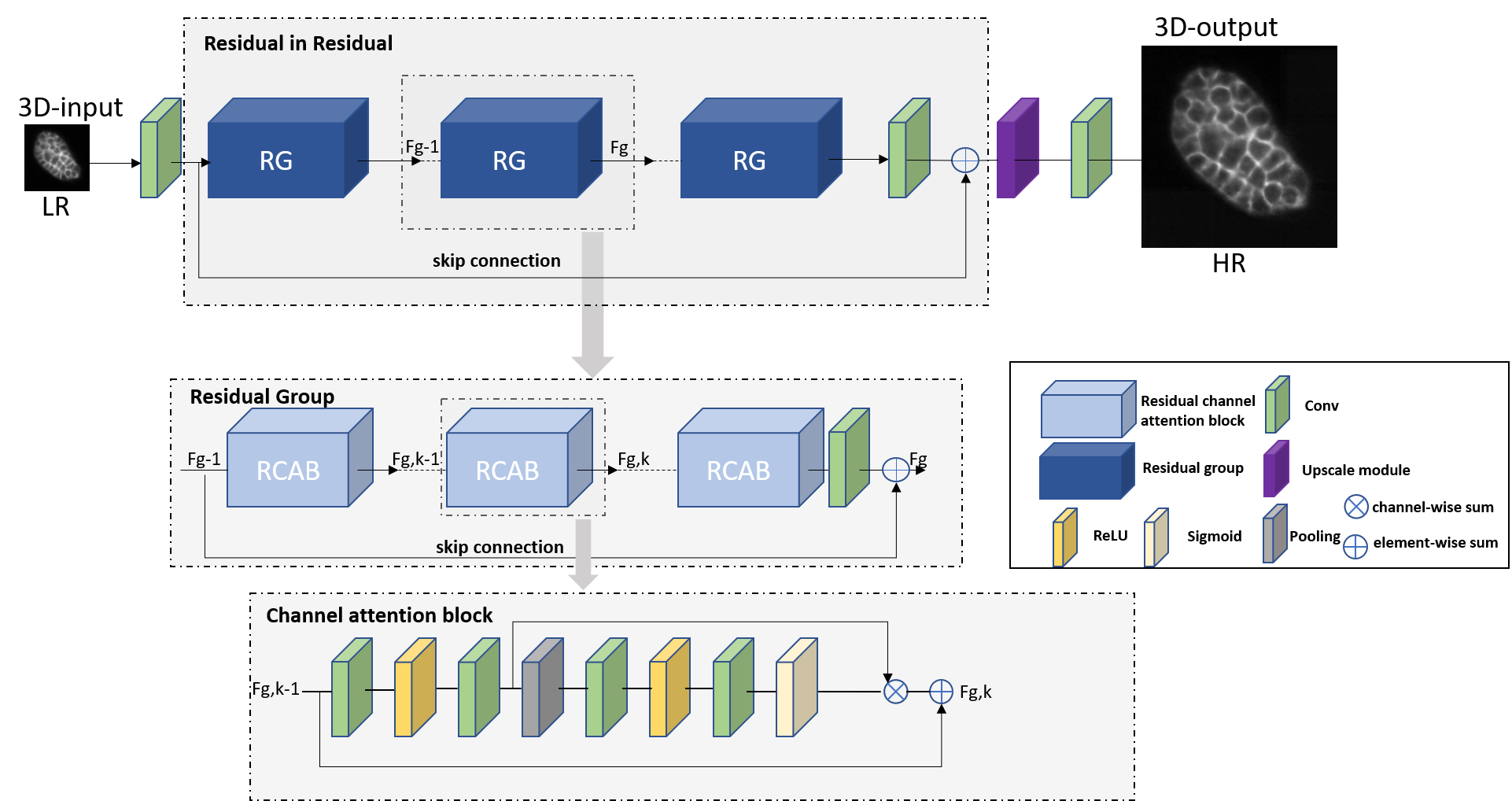
Residual Channel Attention Networks (RCAN1), are deep learning architectures initially designed for 2D super-resolution images, leveraging residual learning and channel attention mechanisms to prioritize high-frequency details. Their hierarchical “residual-in-residual” structure and adaptive channel-wise feature scaling enable superior recovery of fine textures in natural images. Researchers adapted RCAN for 3D fluorescence microscopy data to address challenges in volumetric imaging. This 3D-RCAN2 implementation modifies the original architecture by replacing 2D convolutions with 3D operations, optimizing parameters (e.g., residual groups, channel dimensions) for GPU efficiency, and processing spatiotemporal (4D) data. This adaptation enables denoising and resolution enhancement of volumetric time-lapse microscopy, achieving prolonged live-cell imaging with minimal photo bleaching. By training on paired low/high-quality datasets (e.g., confocal \(\leftrightarrow\) STED or iSIM \(\leftrightarrow\) expansion microscopy), 3D-RCAN restores sub cellular structures, improves lateral and axial resolution, and outperforms existing networks (e.g., CARE)3) in fidelity metrics (e.g., SSIM4 or peak signal to noise ratio). Its applications span fixed and live-cell studies, offering a versatile tool to overcome trade offs between spatiotemporal resolution and phototoxicity in fluorescence microscopy.
Several features of this neural network enable it to handle complex image restoration tasks effectively, as described in the paragraphs below. In later sections, we will employ this model as an example to show you how to undertake AI restoration in fluorescence microscopy.
A.1.1 Residual Learning
3D-RCAN uses a residual learning approach, which means that the network learns the difference (or residual) between the input image and the desired output. Instead of learning the entire image transformation directly, the network focuses on predicting the fine details that need improvement. This makes it easier for the network to capture high-frequency details (like edges and textures) while ignoring unnecessary background information. The network architecture is built using a residual-in-residual structure. This means that within each “residual block” (a unit of processing), there are even smaller “residual blocks.” This hierarchical design improves the network’s ability to learn intricate patterns in the data, allowing for better restoration of fine image details. The network essentially learns to focus on increasingly refined features at different levels of abstraction.
3D-RCAN incorporates skip connections in its architecture. Skip connections are shortcuts that allow the input image to bypass certain network layers and pass directly to later layers. There are long skip connections (which bypass multiple layers) and short skip connections (which skip only a few layers). These connections enable the network to focus on high-frequency information and avoid losing important details that may be “washed out” in deeper layers.
A.1.2 Channel Attention Mechanism
One of the distinctive features of 3D-RCAN is its channel attention mechanism. In any image, different features (such as color or depth in the case of microscopy images) have different levels of influence in the image. The channel attention mechanism allows 3D-RCAN to focus on the most important channels by adaptively adjusting the weight given to each feature channel. This helps the network to enhance high-resolution details in relevant channels while minimizing the influence of less important features.
A.1.3 3D Adaptation for Image Volumes
3D-RCAN is designed to handle not only 2D images but also 3D image volumes. In many microscopy techniques, images are captured as a series of 2D planes stacked together to form a 3D volume. RCAN adapts its structure to process these multi-dimensional data efficiently. By working in 3D, the network can improve both the lateral (XY) and axial (Z) resolution of the image volumes, which is especially important in applications like fluorescence microscopy.
A.1.4 Channel Reduction for Efficient 3D Processing
By reducing channel dimensions before processing and restoring them afterward, the network minimizes redundant computations while retaining essential spatial and structural details. This mechanism enables deeper architectures without overwhelming GPU memory, particularly crucial for large 3D microscopy volumes. Coupled with channel attention, the compressed features are dynamically recalibrated to prioritize high-frequency details, ensuring robust restoration of fine structures like microtubules or mitochondrial membranes. The approach optimizes both training speed and inference performance, validated across synthetic and experimental datasets.
A.2 Overview of the Code and Data
A.2.1 System Requirements
The basic system requirements are:
- Operating System: Windows 10, Linux, or Mac OS
- Python 3.7
- GPU: NVIDIA GPU with CUDA 10.0 and cuDNN 7.6.5
For more information about system requirements, please refer to the 3D-RCAN README.
A.2.2 Installation of Dependencies
3D-RCAN itself does not require installation and installation of the required the dependencies takes few seconds on a typical PC. The installation process involves three main steps:
1. Check system requirements: Ensure your system meets the basic requirements listed above, particularly Python 3.7 and CUDA compatibility.
2. Create a new virtual environment: Set up an isolated Python environment to avoid conflicts with other projects and ensure reproducibility.
3. Install dependencies: Download the repository and install required Python packages using the requirements.txt file provided in the 3D-RCAN respository.
A.2.3 Quick Setup Steps
Clone the repository:
git clone https://github.com/AiviaCommunity/3D-RCAN.gitCreate and activate virtual environment:
# Create virtual environment
python -m venv RCAN3D

# Activate (Windows)
.\\RCAN3D\\Scripts\\activate

# Activate (macOS/Linux)
source RCAN3D/bin/activate
Install dependencies:
pip install -r requirements.txt
For comprehensive installation instructions, please refer to the Dependencies Installation section in the 3D-RCAN README.
A.2.4 Dataset
Custom Data: 3D-RCAN supports 3D data with strict low-quality/high-quality paired training (e.g., noisy/blurred inputs vs. high-SNR/clean GT) . Performance depends on domain alignment between training data (intensity distribution, resolution, noise characteristics) and target applications. The data should follow the format of 3D TIFF stacks (Z-Y-X order).
Example datasets available: You can leverage open-source datasets to obtain paired low-quality and high-quality data, such as the dataset from the 3D-RCAN paper. The 3D RCAN dataset is publicly available on Zenodo. It includes paired low-quality and ground truth (GT) data for diverse applications: denoising mulitple biological structures (actin, ER, Golgi, lysosomes, microtubules, and mitochondria), synthetic blurred phantom spheres with sharp GT, Confocal-to-STED microscopy modality transfer (microtubules, nuclear pores, DNA, and live-cell nuclei), and expansion microscopy (microtubules and mitochondria, pairing synthetic raw images with deconvolved iSIM images). Live-cell test data cover U2OS cells (mitochondria and lysosomes) and Jurkat T cells (EMTB-GFP). Raw data represent inputs (e.g., confocal images, noisy/blurred volumes), while GT corresponds to high-quality outputs (e.g., STED, deconvolved iSIM).
A.2.5 Training
Training a 3D-RCAN model requires a config.json file to specify parameters and data locations.
To initiate training, use the command:
python train.py -c config.json -o /path/to/training/output/dirTraining data can be specified in the config.json file by either:
- Providing paths to folders containing raw and ground truth images (
training_data_dir). - Listing specific pairs of raw and ground truth image files (training_image_pairs).
Numerous other options can be configured in the JSON file, including validation data, model architecture parameters (like num_residual_blocks, num_residual_groups), data augmentation settings, learning rate, loss functions, and metrics. The defaults for num_residual_blocks (3) and num_residual_groups (5) are set to balance performance and hardware constraints, aiming for optimal accuracy on standard GPUs (16-24GB VRAM) without causing memory overflow.
The expected runtime is approximately 5-10 minutes per epoch on a system similar to the tested environment (NVIDIA GeForce GTX 1080 Ti - 11GB) using the example config.json. Training progress and loss values can be monitored using TensorBoard.
For comprehensive details on configuring the config.json file, all available training options, and further instructions, please refer to the Training section in the 3D-RCAN README.
A.2.6 Applying the Model
Trained 3D-RCAN models can be applied using the apply.py script. The script will automatically select the model with the lowest validation loss from the specified model directory.
There are two primary ways to apply a model:
To a single image
python apply.py -m /path/to/model_dir -i input_raw_image.tif -o output.tifTo a folder of images (batch mode)
python apply.py -m /path/to/model_dir
-i /path/to/input_image_dir
-o /path/to/output_image_dir
When processing a folder, ground truth images can also be specified using the -g argument for comparison.
Key command-line arguments include:
-mor--model_dir: Path to the folder containing the trained model (required).-ior--input: Path to the input raw image or folder (required).-oor--output: Path for the output processed image or folder (required).-gor--ground_truth: Path to a reference ground truth image or folder (optional).-bor--bpp: Bit depth of the output image (e.g., 8, 16, 32).-Bor--block_shape: Dimensions (Z,Y,X) for processing large images in blocks.-Oor--block_overlap_shape: Overlap size (Z,Y,X) between blocks.--normalize_output_range_between_zero_and_one: Normalizes output intensity to the [0, 1] range, or to the full bit depth range (e.g., [0, 65535] for 16-bit) when combined with-b.--rescale: Performs affine rescaling to minimize MSE between restored and ground truth images, useful for comparisons similar to CARE methodology.-for--output_tiff_format: Sets the output TIFF format (e.g., “imagej” or “ome”).
For a complete list of all options and detailed explanations, please refer to the Model Apply section in the 3D-RCAN README.
A.3 Denoising Tutorial
A.3.1 Data Preparation
Input Format: 3D TIFF stacks (Z-Y-X order)
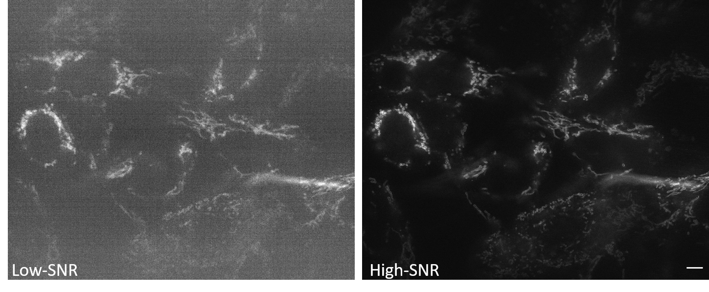
Data Pairs: The example image pairs we employ are shown in Figure A.2 and are available in the denoising section of the data for the 3D-RCAN paper.
Low-SNR Data: Noisy images. Here we use low signal-to-noise ratio data obtained by imaging mitochondria labeled with mEmerald-Tomm20-C-10 in living U2OS cells using instant structured illumination microscopy under low illumination intensities.
High-SNR Ground Truth: Corresponding clean images. Here we use high signal-to-noise ratio and high-resolution data obtained by imaging mitochondria labeled with mEmerald-Tomm20-C-10 in living U2OS cells using instant structured illumination microscopy under high illumination intensities.
Directory Structure: Organize the paired image data as follows.
dataset/
├── train/
│   ├── raw/   # Training noisy data
│   └── gt/    # Training clean data
└── val/
    ├── raw/   # Validation noisy data
    └── gt/    # Validation clean data
The validation data is not necessary for model training, but is an important part of assessing the model quality after training.
A.3.2 Training a Denoising Model
A.3.2.1 Configuration File
Configure the settings file (config_denoise.json) to define the data locations for the training/validation sets and the initial network hyperparameters. An example configuration file is shown below.
{
  "training_data_dir": {
      "raw": "E:\\Denoising\\Tomm20_Mitochondria\\Training\\Raw",
      "gt": "E:\\Denoising\\Tomm20_Mitochondria\\Training\\GT"
  },
  "validation_data_dir": {
      "raw": "E:\\Denoising\\Tomm20_Mitochondria\\Val\\raw",
      "gt": "E:\\Denoising\\Tomm20_Mitochondria\\Val\\gt"
  },
  "num_channels": 32,
  "num_residual_blocks": 3,
  "num_residual_groups": 5,
  "epochs": 100,
  "steps_per_epoch": 256,
  "initial_learning_rate": 1e-4
}
A.3.2.2 Training Command
Run the training using the following command, updating the path to where you have stored the example images as appropriate.
python train.py -c config_denoise.json
-o " E:\\Denoising\\Tomm20_Mitochondria\\output"If you are using a Mac or Linux system, replace the \ in the example paths with /.
A.3.2.3 Training Outputs
The output directory will save the model parameters during the training process. For example, the file weights_092_0.06313289.hdf5 represents the model parameters saved at the 92nd training epoch, with a loss value of 0.06313289.
A.3.3 Applying the Denoising Model
A.3.3.1 Apply Command
To apply the model trainined in the previous section, provide the model (-m), path for the input images (-i), and path for the output denoised images (-o).
python apply.py
  -m "E:\\Denoising\\Tomm20_Mitochondria\\output"
  -i "E:\Denoising\\Tomm20_Mitochondria\\Test\\Raw"
  -o "E:\\Denoising\\Tomm20_Mitochondria\\Test\\Denoised"
A.3.3.2 Output Analysis
Since the output TIFF file is a two-channel ImageJ Hyperstack containing raw and restored images, we can easily compare the denoising effects.
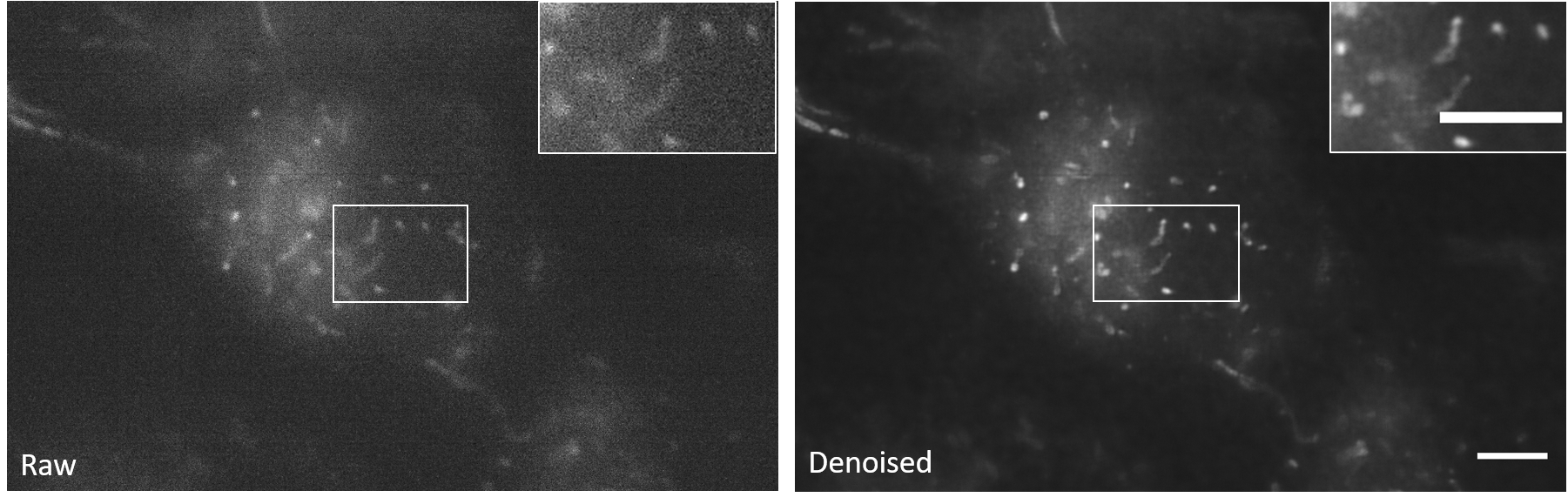
3D-RCAN reconstructs continuous organelle membranes (e.g., mitochondrial cristae) in noisy volumetric data by suppressing stochastic noise, achieving sub-diffraction structural integrity without amplifying high-frequency artifacts or distorting fine textures.
When evaluating the quality of denoised results generated by 3D-RCAN, PSNR (Peak Signal-to-Noise Ratio) and MSE (Mean Squared Error) serve as critical quantitative metrics. PSNR measures the logarithmic relationship between the maximum possible pixel intensity and the distortion introduced during restoration, with higher values indicating better alignment between the restored image and the ground truth (GT). Conversely, MSE calculates the average squared difference between corresponding pixels, where lower values reflect smaller pixel-level errors. For meaningful comparisons, the restored image should exhibit a higher PSNR and lower MSE relative to the raw input when both are evaluated against the GT. This directly quantifies the model’s ability to enhance resolution while minimizing deviations from the true signal.
You can calculate PSNR and MSE with the formulas below, where \(m\), \(n\), and \(p\) are the dimensions of the 3D image. \(I_{\text{raw}}(i,j,k)\) is the intensity value of the raw image at position \((i,j,k)\) and \(I_{\text{GT}}(i,j,k)\) is the intensity value of the ground truth image at position \((i,j,k)\).
\[ \text{MSE} = \frac{1}{m n p} \sum_{i=0}^{m-1} \sum_{j=0}^{n-1} \sum_{k=0}^{p-1} [I_{\text{raw}}(i,j,k)-I_{\text{GT}}(i,j,k)]^2 \tag{A.1}\]
\[ \text{PSNR} = 10 \cdot \log_{10}\left(\frac{\text{MAX}_I^2}{\text{MSE}}\right) \tag{A.2}\]
We recommend intensity normalization across raw, restored, and GT images (e.g., scaling to \([0,1]\)) to avoid metric distortions. For heterogeneous samples, compute localized metrics within regions of interest (e.g., cell membranes vs. cytoplasm) to identify performance variations. Note that while high PSNR/MSE improvements generally correlate with perceptual quality, they should complement visual inspection and task-specific validations (e.g., downstream analysis accuracy). Always verify that the model’s output preserves biological relevance—metrics alone cannot capture context-specific artifacts or over-smoothing.
A.3.4 Further Denoising Guidance
To improve the performance of the 3D-RCAN model when unsatisfied with denoising results, we recommend starting by tuning hyperparameters in the config.json file. Start by adjusting the model architecture parameters to balance computational constraints and feature extraction capabilities. For instance, increasing num_channels (default:32) enhances the network’s capacity to learn complex features but requires more GPU memory. If limited by hardware, reducing it to 16-24 while moderately increasing num_residual_groups (default:5) or num_residual_blocks per group (default:3) could maintain depth without overwhelming resources. The channel_reduction ratio (default:8) for attention mechanisms can be lowered to 4-6 to amplify the model’s sensitivity to channel-wise dependencies, though this should be validated using metrics to avoid overfitting.
Training dynamics can be optimized by revisiting the initial_learning_rate (default:1e-4). If training loss plateaus or fluctuates, gradually lowering it to 1e-5 stabilizes convergence, while aggressive learning rates (e.g., 5e-4) might accelerate early training but risk divergence. Switching the loss function from MAE (robust to noise) to MSE could prioritize pixel-level accuracy for high-frequency details, especially when ground truth data has sharp structures. Extending training epochs beyond the default 300—coupled with early stopping based on validation loss—helps the model capture subtle patterns in volumetric data.
Data-related parameters require careful calibration. Enabling data_augmentation (default:True) remains vital for small datasets to simulate variations in microscopy imaging, but it can be disabled for large, diverse datasets to speed up training. The intensity_threshold (default:0.25) and area_ratio_threshold (default:0.5) act as filters for low-quality patches. Raising the intensity threshold to 0.3-0.4 suppresses noisy backgrounds, while lowering the area ratio to 0.3-0.4 accommodates sparse biological structures like microtubules. For validation, always specify a dedicated validation_data_dir to monitor generalization and prevent overfitting.
Finally, hardware limitations can be mitigated by reducing block_shape dimensions during inference or simplifying the model architecture. Experiment iteratively: establish a baseline with default settings, then progressively scale model complexity while tracking validation metrics like PSNR/SSIM. Consider hybrid strategies, such as combining MAE loss with SSIM regularization (a loss penalty using SSIM to preserve structural fidelity and prevent over-smoothing) or dynamic learning rate schedules, to adapt to specific data characteristics. Always validate changes against biologically relevant structures in your test set, as quantitative metrics alone may not reflect practical image quality for microscopy analysis.
A.4 Deconvolution Tutorial
A.4.1 Data Preparation
Input Format: 3D TIFF stacks (Z-Y-X order)
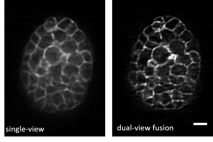
Data Pairs: The example image pairs we employ here are shown in Figure A.4 and are available in the ‘DL Decon’ section of DeAbePlusData.
Input (Raw): Low-quality, blurry 3D images with PSF such as single-view volumetric images acquired via diSPIM (0.8 NA \(\times\) 0.8 NA optics), with voxel size 0.1625 \(\times\) 0.1625 \(\times\) 1.0 µm
Ground Truth (GT): High-quality, non-blurry 3D images such as dual-view joint deconvolution-reconstructed volumes (fusion of both diSPIM views), with isotropic resolution.
Directory Structure: Organize data as follows.
dataset/
├── train/
│   ├── raw/   # Training raw data
│   └── gt/    # Training label data
└── val/
    ├── raw/   # Validation raw data
    └── gt/    # Validation label data
The validation data is not necessary for model training, but is an important part of assessing the model quality after training.
A.4.2 Training a Deconvolution Model
A.4.2.1 Configuration File
Configure the settings file (config_decon.json) to define the data locations for the training/validation sets and the initial network hyper-parameters.
{
  "training_data_dir": {
      "raw": "E:\\data_decon\\Decon_Training_Data\\Raw",
      "gt":"E:\\data_decon\\Decon_Training_Data\\gt"
  },
  "validation_data_dir": {
      "raw":"E:\\data_decon\\Decon_val_Data\\Raw",
      "gt": "E:\\data_decon\\Decon_val_Data\\gt"
  },
  "num_channels": 32,
  "num_residual_blocks": 3,
  "num_residual_groups": 5,
  "epochs": 200,
  "steps_per_epoch": 256,
  "initial_learning_rate": 1e-4
}
A.4.2.2 Training Command
Run the training using the following command, updating the path to where you have stored the example images as appropriate.
python train.py -c config_decon.json -o "E:\\data_decon\\model_output"If you are using a Mac or Linux system, replace the \ in the example paths with /.
A.4.2.3 Training Outputs:
The output directory will save the model parameters during the training process. For example, the file weights_092_0.06313289.hdf5 represents the model parameters saved at the 92nd training epoch, with a loss value of 0.06313289.
A.4.3 Applying the Deconvolution Model
A.4.3.1 Apply Command
To apply the model trainined in the previous section, provide the model (-m), path for the input images (-i), and path for the output denoised images (-o).
python apply.py
  -m "E:\\data_decon\\model_output"
  -i "E:\\data_decon\\Decon_val_Data\\Raw"
  -o "E:\\data_decon\\Decon_val_Data\\deconvolved"
A.4.3.2 Output Analysis
Since the output TIFF file is a two-channel ImageJ Hyperstack containing raw and restored images, we can easily compare the deconvolved effects.
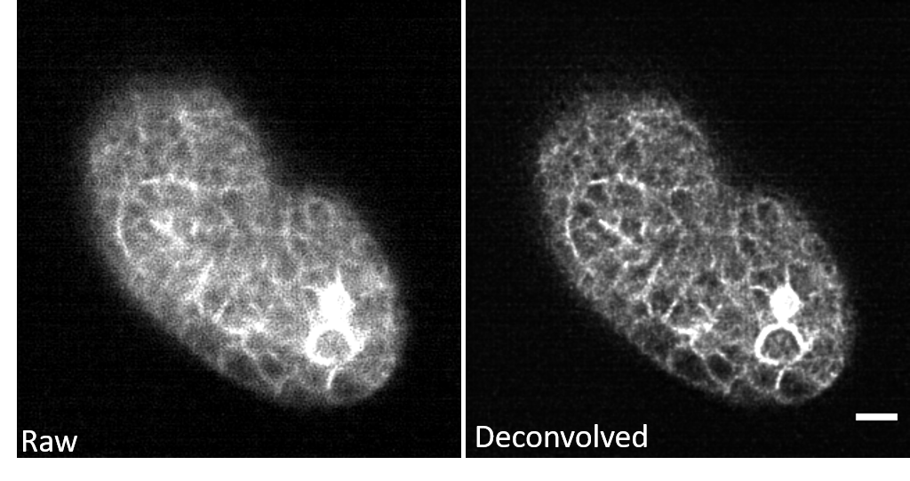
3D-RCAN corrects out-of-focus blur in GFP-labeled C. elegans embryos, resolving densely packed microtubule arrays within mitotic spindles and restoring cortical membrane contours obscured by optical scattering in thick embryonic samples, without introducing grid-like artifacts typical of Fourier-based deconvolution.
Refer to Section A.3.3.2 for baseline validation metrics. Compare with classical methods (e.g., Richardson5 -Lucy6 Deconvolution).
A.4.4 Further Deconvolution Guidance
Refer to Section A.3.4 for general guidance. For deconvolution, use a lightweight attention mechanism (\(\leq\) 3 channel reduction steps) to avoid over-smoothing high-frequency structures.
A.5 Aberration Correction Tutorial
A.5.1 Data Preparation
Input Format: 3D TIFF stacks (Z-Y-X order)
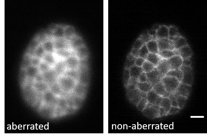
Data Pairs: The sample image pairs employed here were C. elegans embryos expressing a GFP marker , as shown in Figure A.6. You can find these examples in the ‘DL DeAbe’ section of the DeAbePlusData.
Aberrated Input Data: Artificially degraded images, corrupted by synthetic aberrations modeled via Zernike polynomials (modes 1–7, defocus coefficient \(\leq\) 1.5 rad, other modes \(\leq\) 0.5 rad) and Poisson noise. Degradation is applied to shallow-layer ground truth using the physical forward model.
High-Quality Label Data: Directly acquired shallow-layer images serve as ground truth, validated by their proximity to the objective lens (minimal inherent aberrations).
Directory Structure: Organize data as follows.
dataset/
├── train/
│   ├── raw/   # Training aberrated data
│   └── gt/    # Training label data
└── val/
    ├── raw/   # Validation aberrated data
    └── gt/    # Validation label data
The validation data is not necessary for model training, but is an important part of assessing the model quality after training.
A.5.2 Training an Aberration Correction Model
A.5.2.1 Configuration File
Configure the settings file (config_deabe.json) to define the data locations for the training/validation sets and the initial network hyperparameters.
{
  "training_data_dir": {
      "raw": "E:\\data_aberration\\CropForTraining_ab\\Aberrated",
      "gt":"E:\\data_aberration\\CropForTraining_ab\\GT"
  },
  "validation_data_dir": {
      "raw":"E:\\data_aberration\\CropForTraining_ab\\Validation\\Aberrated",
      "gt": "E:\\data_aberration\\CropForTraining_ab\\Validation\\GT"
  },
  "num_channels": 32,
  "num_residual_blocks": 3,
  "num_residual_groups": 5,
  "epochs": 100,
  "steps_per_epoch": 100,
  "initial_learning_rate": 1e-4
}
A.5.2.2 Training Command
Run the training using the following command, updating the path to where you have stored the example images as appropriate.
python train.py -c config_deabe.json
-o " E:\\DeAbe\\Train\\output"If you are using a Mac or Linux system, replace the \ in the example paths with /.
A.5.2.3 Training Outputs:
The output directory will save the model parameters during the training process. For example, the file weights_092_0.06313289.hdf5 represents the model parameters saved at the 92nd training epoch, with a loss value of 0.06313289.
A.5.3 Applying the Aberration Correction Model
A.5.3.1 Apply Command
To apply the model trainined in the previous section, provide the model (-m), path for the input images (-i), and path for the output denoised images (-o).
python apply.py
  -m "E:\\DeAbe\\Train\\output"
  -i "E:\DeAbe\\Test\\Raw"
  -o "E:\\DeAbe\\Test\\Deabrrated"
A.5.3.2 Output Analysis
Since the output TIFF file is a two-channel ImageJ Hyperstack containing raw and restored images, we can easily compare the de-aberration effects.
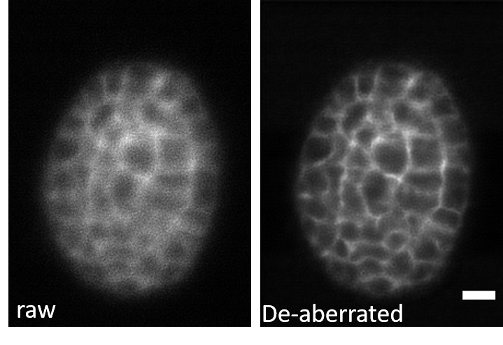
3D-RCAN effectively corrects system-induced optical aberrations in GFP-labeled C. elegans embryos. The de-aberrated image restores spatially ordered structures obscured by asymmetric blur in the raw data, while suppressing background granularity and enhancing signal-to-background contrast.
Refer to Section A.3.3.2 for baseline validation metrics. For aberration correction validation, analyze Fourier spectra to assess restored spatial symmetry and high-frequency energy, quantify wavefront errors via phase retrieval or bead-based PSF measurements, and evaluate intensity uniformity/edge sharpness across volumes.
A.5.4 Further Aberration Correction Guidance
Refer to Section A.3.4 for basic guidance. Prioritize RCAB layers with wider receptive fields (kernel size \(\leq 5^3\)) to capture large-scale distortion patterns.
A.6 Resolution Enhancement Tutorial
A.6.1 Data Preparation
Input Format: 3D TIFF stacks (Z-Y-X order)
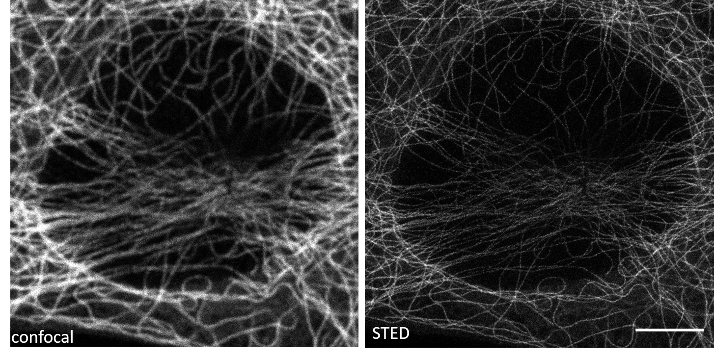
Data Pairs: The example image pairs we employ are shown in Figure A.8. You can find these examples in the ‘confocal_2_STED’ section of the data for the 3D-RCAN paper.
Raw data: The “raw” data here refers to the original confocal microscopy images of the fixed mouse embryonic fibroblast (MEF) cells, specifically focusing on the microtubules. These images are acquired directly from the confocal microscope without any further processing or enhancement. They represent the initial, unaltered state of the microtubule structures as captured by the confocal microscope.
Ground Truth (GT) data: The “ground truth” (GT) data consists of the high-resolution STED (Stimulated Emission Depletion) microscopy images of the same fixed MEF cells, again focusing on the microtubules.
Directory Structure: Organize data as follows.
dataset/
├── train/
│   ├── raw/   #confocal data
│   └── gt/    #STED data
└── val/
    ├── raw/   # confocal data
    └── gt/    # STED data
The validation data is not necessary for model training, but is an important part of assessing the model quality after training.
A.6.2 Training a Resolution Enhancement Model
A.6.2.1 Configuration File
Configure the settings file (config_sr.json) to define the data locations for the training/validation sets and the initial network hyper-parameters.
{
  "training_data_dir": {
      "raw": "E:\\Confocal_2_STED\\Microtubule\\Training\\raw",
      "gt": "E:\\Confocal_2_STED\\Microtubule\\Training\\gt1"

  },

  "num_channels": 32,
  "num_residual_blocks": 3,
  "num_residual_groups": 5,
  "epochs": 100,
  "steps_per_epoch": 256,
  "initial_learning_rate": 1e-4
}
A.6.2.2 Training Command
Run the training using the following command, updating the path to where you have stored the example images as appropriate.
python train.py
-c config_ex.json
-o "E:\\Confocal_2_STED\\Microtubule\\Training\\output"If you are using a Mac or Linux system, replace the \ in the example paths with /.
A.6.3 Applying the Resolution Enhancement Model
A.6.3.1 Apply Command
To apply the model trainined in the previous section, provide the model (-m), path for the input images (-i), and path for the output denoised images (-o).
 python apply.py
 -m "E:\\Confocal_2_STED\\Microtubule\\Training\\output"
 -i "E:\DATA_for_3dRCAN\Confocal_2_STED\Microtubule\test\"
 -o "E:\\Confocal_2_STED\\Microtubule\\test\output\\"
A.6.3.2 Output Analysis
Since the output TIFF file is a two-channel ImageJ Hyperstack containing raw and restored images, we can easily investigate the extent of resolution enhancement.
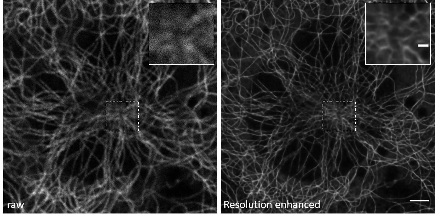
The model resolves densely packed microtubule intersections and eliminates axial blur in confocal-derived volumes, restoring filament topology to near-STED resolution.
Refer to Section A.3.3.2 for baseline validation metrics. Check for artifacts in Z-stack transitions and consistency in organelle morphology.
A.6.4 Further Resolution Enhancement Guidance
Refer to Section A.3.4 for basic guidance. Optimize residual groups (e.g., increase from 5 to 10) and channel dimensions (\(\leq 64\)) to handle spatially variant upsampling.